- Stokes' theorem
-
For the equation governing viscous drag in fluids, see Stokes' law.
In differential geometry, Stokes' theorem (or Stokes's theorem, also called the generalized Stokes' theorem) is a statement about the integration of differential forms on manifolds, which both simplifies and generalizes several theorems from vector calculus. Lord Kelvin first discovered the result and communicated it to George Stokes in July 1850.[1][2] Stokes set the theorem as a question on the 1854 Smith's Prize exam, which led to the result bearing his name.[2]
Contents
Introduction
The fundamental theorem of calculus states that the integral of a function f over the interval [a, b] can be calculated by finding an antiderivative F of f:
Stokes' theorem is a vast generalization of this theorem in the following sense.
- By the choice of F,
 . In the parlance of differential forms, this is saying that f(x) dx is the exterior derivative of the 0-form, i.e. function, F: in other words, that dF = f dx. The general Stokes theorem applies to higher differential forms ω instead of F.
 - A closed interval [a, b] is a simple example of a one-dimensional manifold with boundary. Its boundary is the set consisting of the two points a and b. Integrating f over the interval may be generalized to integrating forms on a higher-dimensional manifold. Two technical conditions are needed: the manifold has to be orientable, and the form has to be compactly supported in order to give a well-defined integral.
- The two points a and b form the boundary of the open interval. More generally, Stokes' theorem applies to oriented manifolds M with boundary. The boundary ∂M of M is itself a manifold and inherits a natural orientation from that of the manifold. For example, the natural orientation of the interval gives an orientation of the two boundary points. Intuitively, a inherits the opposite orientation as b, as they are at opposite ends of the interval. So, "integrating" F over two boundary points a, b is taking the difference F(b) − F(a).
In even simpler terms, one can consider that points can be thought of as the boundaries of curves, that is as 0-dimensional boundaries of 1-dimensional manifolds. So, just like one can find the value of an Integral (f = dF) over a 1-dimensional manifolds ([a,b]) by considering the anti-derivative (F) at the 0-dimensional boundaries ([a,b]), one can generalize the fundamental theorem of calculus, with a few additional caveats, to deal with the value of integrals (dω) over n-dimensional manifolds (Ω) by considering the anti-derivative (ω) at the (n-1)-dimensional boundaries (dΩ) of the manifold.
So the fundamental theorem reads:
General formulation
Let Ω be an oriented smooth manifold of dimension n and let
 be an n-differential form that is compactly supported on Ω. First, suppose that α is compactly supported in the domain of a single, oriented coordinate chart {U, φ}. In this case, we define the integral of over Ω as
i.e., via the pullback of α to Rn.
More generally, the integral of
over Ω is defined as follows: Let {ψi} be a partition of unity associated with a locally finite cover {Ui, φi} of (consistently oriented) coordinate charts, then define the integralwhere each term in the sum is evaluated by pulling back to Rn as described above. This quantity is well-defined; that is, it does not depend on the choice of the coordinate charts, nor the partition of unity.
Stokes' theorem reads: If ω is an (n − 1)-form with compact support on Ω and
 denotes the boundary of Ω with its induced orientation, then
 A "normal" integration manifold (here called D instead of Ω) for the special case n=2
Here
 is the exterior derivative, which is defined using the manifold structure only. On the r.h.s., a circle is sometimes used within the integral sign to stress the fact that the (n-1)-manifold is closed.[3] The r.h.s. of the equation is often used to formulate integral laws; the l.h.s. then leads to equivalent differential formulations (see below).
The theorem is often used in situations where Ω is an embedded oriented submanifold of some bigger manifold on which the form ω is defined.
A proof becomes particularly simple if the submanifold Ω is a so-called "normal manifold", as in the figure on the r.h.s., which can be segmented into vertical stripes (e.g. parallel to the xn direction), such that after a partial integration concerning this variable, nontrivial contributions come only from the upper and lower boundary surfaces (coloured in yellow and red, respectively), where the complementary mutual orientations are visible through the arrows.
Topological reading; integration over chains
Let M be a smooth manifold. A smooth singular k-simplex of M is a smooth map from the standard simplex in Rk to M. The free abelian group, Sk, generated by singular k-simplices is said to consist of singular k-chains of M. These groups, together with boundary map, ∂, define a chain complex. The corresponding homology (resp. cohomology) is called the smooth singular homology (resp. cohomology) of M.
On the other hand, the differential forms, with exterior derivative, d, as the connecting map, form a cochain complex, which defines de Rham cohomology.
Differential k-forms can be integrated over a k-simplex in a natural way, by pulling back to Rk. Extending by linearity allows one to integrate over chains. This gives a linear map from the space of k-forms to the k-th group in the singular cochain, Sk*, the linear functionals on Sk. In other words, a k-form
 defines a functional
on the k-chains. Stokes' theorem says that this is a chain map from de Rham cohomology to singular cohomology; the exterior derivative, d, behaves like the dual of ∂ on forms. This gives a homomorphism from de Rham cohomology to singular cohomology. On the level of forms, this means:
- closed forms, i.e.,
 , have zero integral over boundaries, i.e. over manifolds that can be written as
  , and
, and - exact forms, i.e.,
 , have zero integral over cycles, i.e. if the boundaries sum up to the empty set:
  .
.
De Rham's theorem shows that this homomorphism is in fact an isomorphism. So the converse to 1 and 2 above hold true. In other words, if {ci} are cycles generating the k-th homology group, then for any corresponding real numbers, {ai}, there exist a closed form,
, such that:and this form is unique up to exact forms.
Underlying principle
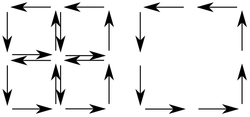
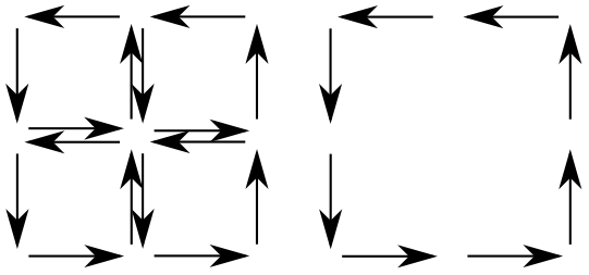
To simplify these topological arguments, it is worthwhile to examine the underlying principle by considering an example for d = 2 dimensions. The essential idea can be understood by the diagram on the left, which shows that, in an oriented tiling of a manifold, the interior paths are traversed in opposite directions; their contributions to the path integral thus cancel each other pairwise. As a consequence, only the contribution from the boundary remains. It thus suffices to prove Stokes' theorem for sufficiently fine tilings (or, equivalently, simplices), which usually is not difficult.
Special cases
The general form of the Stokes theorem using differential forms is more powerful and easier to use than the special cases. Because in Cartesian coordinates the traditional versions can be formulated without the machinery of differential geometry they are more accessible, older and have familiar names. The traditional forms are often considered more convenient by practicing scientists and engineers but the non-naturalness of the traditional formulation becomes apparent when using other coordinate systems, even familiar ones like spherical or cylindrical coordinates. There is potential for confusion in the way names are applied, and the use of dual formulations.
Kelvin–Stokes theorem
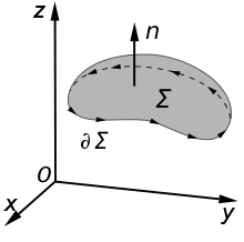 An illustration of the Kelvin–Stokes theorem, with surface Σ, its boundary
 and the "normal" vector n.
This is a (dualized) 1+1 dimensional case, for a 1-form (dualized because it is a statement about vector fields). This special case is often just referred to as the Stokes' theorem in many introductory university vector calculus courses and as used in physics and engineering. It is also sometimes known as the curl theorem.
The classical Kelvin–Stokes theorem:
which relates the surface integral of the curl of a vector field over a surface Σ in Euclidean three-space to the line integral of the vector field over its boundary, is a special case of the general Stokes theorem (with n = 2) once we identify a vector field with a 1 form using the metric on Euclidean three-space. The curve of the line integral, ∂Σ, must have positive orientation, meaning that dr points counterclockwise when the surface normal, dΣ, points toward the viewer, following the right-hand rule.
One consequence of the formula is that the field lines of a vector field with zero curl cannot be closed contours.
The formula can be rewritten as:
where P, Q and R are the components of F.
These variants are frequently used:
In electromagnetism
Two of the four Maxwell equations involve curls of 3-D vector fields and their differential and integral forms are related by the Kelvin–Stokes theorem. Caution must be taken to avoid cases with moving boundaries: the partial time derivatives are intended to exclude such cases. If moving boundaries are included, interchange of integration and differentiation introduces terms related to boundary motion not included in the results below:
Name Differential form Integral form (using Kelvin–Stokes theorem plus relativistic invariance,  )
)Maxwell-Faraday equation
Faraday's law of induction:
 (with C and S not necessarily stationary)
Ampère's law
(with Maxwell's extension):
 (with C and S not necessarily stationary)
The above listed subset of Maxwell's equations are valid for electromagnetic fields expressed in SI units. In other systems of units, such as CGS or Gaussian units, the scaling factors for the terms differ. For example, in Gaussian units, Faraday's law of induction and Ampère's law take the forms[4][5]
respectively, where c is the speed of light in vacuum.
Divergence theorem
Likewise the Ostrogradsky-Gauss theorem (also known as the Divergence theorem or Gauss's theorem)
is a special case if we identify a vector field with the n−1 form obtained by contracting the vector field with the Euclidean volume form.
Green's theorem
Green's theorem is immediately recognizable as the third integrand of both sides in the integral in terms of P, Q, and R cited above.
Notes
- ^ Olivier Darrigol,Electrodynamics from Ampere to Einstein, p. 146,ISBN 0198505930 Oxford (2000)
- ^ a b Spivak (1965), p. vii, Preface.
- ^ For mathematicians this fact is known, therefore the circle is redundant and often left away. However, one should keep in mind here that in thermodynamics, where frequently expressions as
 appear (wherein the total derivative, see below, should not be mixed-up with the exterior one), the integration path W is a one-dimensional closed line on a much higher-dimensional manifold. I.e. in a thermodynamic application, where U is a function of the temperature α1: = T, the volume
  and the electrical polarization α3: = P of the sample, one has
  and the circle is really necessary, e.g. if one considers the differential consequences of the integral postulate
- ^ J.D. Jackson, Classical Electrodynamics, 2nd Ed (Wiley, New York, 1975).
- ^ M. Born and E. Wolf, Principles of Optics, 6th Ed. (Cambridge University Press, Cambridge, 1980).
Further reading
- Joos, Georg. Theoretische Physik. 13th ed. Akademische Verlagsgesellschaft Wiesbaden 1980. ISBN 3-400-00013-2
- Katz, Victor J. (May 1979), "The History of Stokes' Theorem", Mathematics Magazine 52 (3): 146–156, http://links.jstor.org/sici?sici=0025-570X(197905)52%3A3%3C146%3ATHOST%3E2.0.CO%3B2-O
- Marsden, Jerrold E., Anthony Tromba. Vector Calculus. 5th edition W. H. Freeman: 2003.
- Lee, John. Introduction to Smooth Manifolds. Springer-Verlag 2003. ISBN 978-0-387-95448-6
- Rudin, Walter (1976), Principles of Mathematical Analysis, New York: McGraw-Hill, ISBN 0-07-054235-X
- Spivak, Michael (1965), Calculus on Manifolds: A Modern Approach to Classical Theorems of Advanced Calculus, HarperCollins, ISBN 978-0-8053-9021-6
- Stewart, James. Calculus: Concepts and Contexts. 2nd ed. Pacific Grove, CA: Brooks/Cole, 2001.
- Stewart, James. Calculus: Early Transcendental Functions. 5th ed. Brooks/Cole, 2003.
External links
Categories:- Differential topology
- Differential forms
- Duality theories
- Integration on manifolds
- Theorems in calculus
- Theorems in geometry

![\int_{[a, b]} f(x)\,\mathrm{d}x = \int_{[a, b]} \mathrm{d}F = \int_{\{a\}^- \cup \{b\}^+} F = F(b) - F(a).](d/3fd230fcd1a533755a599f99ccf0e8a2.png)


Wikimedia Foundation. 2010.