- Multivariate stable distribution
-
multivariate stable Probability density function
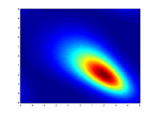
Heatmap showing a Multivariate (bivariate) stable distribution with α = 1.1parameters: ![\alpha \in (0,2]](4/944e6f204ae8b4999ec296da3cd2c905.png) — exponent
— exponent
 - shift/location vector
Λ(s) - a spectral finite measure on the spheresupport: 
pdf: (no analytic expression) cdf: (no analytic expression) variance: Infinite when α < 2 cf: see text The multivariate stable distribution is a multivariate probability distribution that is a multivariate generalisation of the univariate stable distribution. The multivariate stable distribution defines linear relations between stable distribution marginals.[clarification needed] In the same way as for the univariate case, the distribution is defined in terms of its characteristic function.
The multivariate stable distribution can also be thought as an extension of the multivariate normal distribution. It has parameter, α, which is defined over the range 0 < α ≤ 2, and where the case α = 2 is equivalent to the multivariate normal distribution. It has an additional skew parameter that allows for non-symmetric distributions, where the multivariate normal distribution is symmetric.
Contents
Definition
Let S be the unit sphere in
 . For a random variable, X, it has a multivariate stable distribution and the notation X∼S(α,Λ,δ) is used, if the joint characteristic function of X is[1]
where 0 < α < 2, and
This is essentially the result of Feldheim,[2] that any stable random vector can be characterized by a spectral measure Λ (a finite measure on S) and a shift vector
 .
.Parametrization using projections
Another way to describe a stable random vector is in terms of projections. For any vector u, the projection uTX is univariate α − stable with some skewness β(u), scale γ(u) and some shift δ(u). The notation
 is used if uTX is stable with
 for every
  . This is called the projection parameterization.
The spectral measure determines the projection parameter functions by:
Special cases
There are four special cases where the multivariate characteristic function takes a simpler form. Define the characteristic function of a stable marginal as
Isotropic multivariate stable distribution
The characteristic function is
 The spectral measure is continuous and uniform, leading to radial/isotropic symmetry.[3]
Elliptically contoured multivariate stable distribution
Elliptically contoured m.v. stable distribution is a special symmetric case of the multivariate stable distribution. If X is α-stable and elliptically contoured, then it has joint characteristic function Eexp(iuTX) = exp{ − (uTΣu)α / 2 + iuTδ)} for some positive definite matrix Σ and shift vector
. Note the relation to characteristic function of the multivariate normal distribution: Eexp(iuTX) = exp{ − (uTΣu) + iuTδ)}. In other words, when α = 2 we get the characteristic function of the multivariate normal distribution.Independent components
The marginals are independent with Xj∼S(α,βj,γj,δj), then the characteristic function is
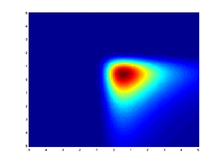
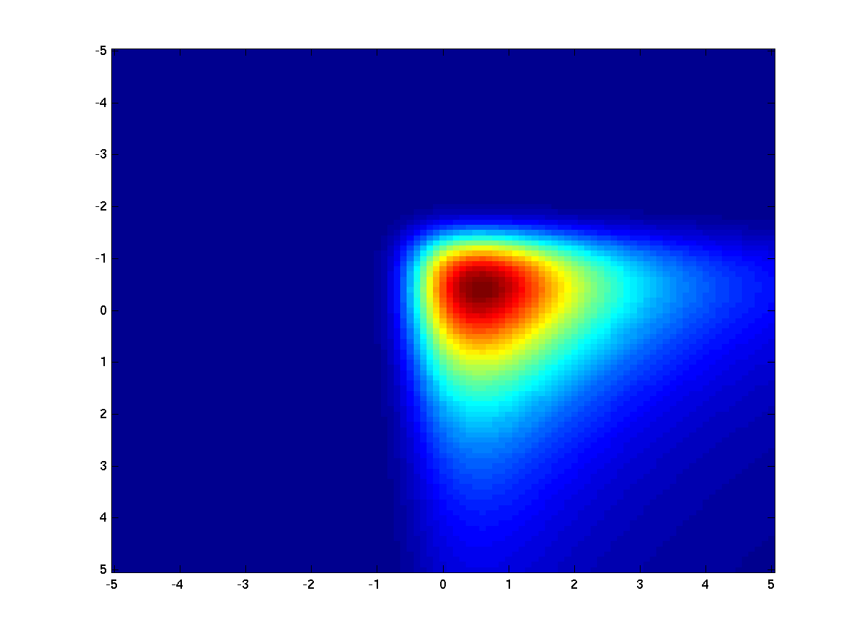
Heatmap showing a multivariate (bivariate) independent stable distribution with α = 1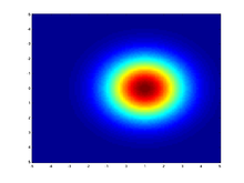
Heatmap showing a multivariate (bivariate) independent stable distribution with α = 2.Discrete
If the spectral measure is discrete with mass λj at
 the characteristic function is
Linear properties
if
is d-dim, and A is a m x d matrix,  then AX + b is m dim. α-stable with scale function
  , skewness function
  , and location function
Inference in the independent component model
Recently[4] it was shown how to compute inference in closed-form in a linear model (or equivalently a factor analysis model),involving independent component models.
More specifically, let
 be a set of i.i.d. unobserved univariate drawn from a stable distribution. Given a known linear relation matrix A of size
  , the observation
  are assumed to be distributed as a convolution of the hidden factors Xi.
  . The inference task is to compute the most probable Xi, given the linear relation matrix A and the observations Yi. This task can be computed in closed-form in O(n3).
An application for this construction is multiuser detection with stable, non-Gaussian noise.
Resources
- Mark Veillette's stable distribution matlab package http://math.bu.edu/people/mveillet/research.html
- The plots in this page where plotted using Danny Bickson's inference in linear-stable model Matlab package: http://www.cs.cmu.edu/~bickson/stable
Notes
- ^ Multivariate stable densities and distribution functions: general and elliptical case, BundesBank Conference, Eltville, Germany, 11 November 2005
- ^ Feldheim, E. (1937). Etude de la stabilit´e des lois de probabilit´e . Ph. D. thesis, Facult´e des Sciences de Paris, Paris, France.
- ^ User manual for STABLE 5.1 Matlab version, Robust Analytics inc.[Full citation needed]
- ^ D. Bickson and C. Guestrin. Inference in linear models with multivariate heavy-tails. In Neural Information Processing Systems (NIPS) 2010, Vancouver, Canada, Dec. 2010. http://www.cs.cmu.edu/~bickson/stable/
Categories:- Multivariate continuous distributions


![\omega(u|\alpha,\beta) =
\begin{cases}|u|^\alpha\left[1-i \beta(\tan \tfrac{\pi\alpha}{2})\mathbf{sign}(u)\right]& \alpha \ne 1\\
|u|\left[1+i \beta \tfrac{2}{\pi} \mathbf{sign}(u)\ln |u|\right] & \alpha = 1\end{cases}](5/bf534e1941cd6499cf13664c1bfc45a5.png)


Wikimedia Foundation. 2010.