- Scale (map)
-
The scale of a map is defined as the ratio of a distance on the map to the corresponding distance on the ground.
If the region of the map is small enough for the curvature of the Earth to be neglected, then the scale may be taken as a constant ratio over the whole map. (A town plan would be an example). For maps covering larger areas, or the whole Earth, it is essential to use a map projection[1][2] from the sphere (or ellipsoid) to the plane. Such projections inevitably involve distortion and the scale can no longer be considered as constant. It is then necessary to introduce the concept of a variable point scale (or particular scale) which is defined as the ratio of the length of a small line element emanating from a point on the map to the length of the corresponding line element on the surface of the Earth. In general the point scale will vary with the position of the point and also the direction of the line element.
Tissot's indicatrix is often used to illustrate the variation of point scale. In the study of point scale it is convenient to define the projection formulae in such a way that the scale is unity, or nearly so, on some lines (or points) of the resulting map projection.
Clearly such a map projection must be comparable to the size of the Earth and, in order to represent it on a small sheet of paper, it must be scaled down by a constant ratio known as the representative fraction (RF) or principal scale. Thus we have to differentiate two uses of the word scale: the variable point scale inherent in the projection and the constant scale involved in the reduction to the printed (or screen) map.
The terminology of scales
Map scales may be expressed in words (a lexical scale), as a ratio, or as a fraction. Examples are:
-
- 'one centimetre to one hundred metres' or 1:10,000 or 1/10,000
- 'one inch to one mile' or 1:63,360 or 1/63,360
- 'one centimetre to one thousand kilometres' or 1:100,000,000 or 1/100,000,000. (The ratio would usually be abbreviated to 1:100M).
In addition to the above many maps carry one or more (graphical) bar scales. For example some British maps presently (2009) use three bar scales for kilometres, miles and nautical miles.
A lexical scale on a recently published map, in a language known to the user, may be easier for a non-mathematician to visualise than a ratio: if the scale is an inch to two miles and he can see that two villages are about two inches apart on the map then it is easy to work out that they are about four miles apart on the ground.
On the other hand, a lexical scale may cause problems if it expressed in a language that the user does not understand or in obsolete or ill-defined units. On the other hand ratios and fractions may be more acceptable to the numerate user since they are immediately accessible in any language. For example a scale of one inch to a furlong (1:7920) will be understood by many older people in countries where Imperial units used to be taught in schools. But a scale of one pouce to one league may be about 1:144,000 but it depends on the cartographer's choice of the many possible definitions for a league, and only a minority of modern users will be familiar with the units used.
Maps are often described as small scale, typically for world maps or large regional maps, showing large areas of land on a small space, or large scale, showing smaller areas in more detail, typically for county maps or town plans. The town plan might be on a scale of 1:10,000 and the world map might be on a scale of 1:100,000,000. There is no hard and fast dividing line between "small" and "large" scales.
For maps covering large areas, a noticeable distortion may arise from the mapmaker's attempt to map the earth's curved surface onto a flat sheet of paper. The type of distortion will depend on the map projection used. In this case the true scale will vary over the area of the map, and the stated map scale will only be an approximation. This is discussed in great detail below.
Large scale maps with curvature neglected
The region over which the earth can be regarded as flat depends on the accuracy of the survey measurements. If measured only to the nearest metre, then curvature is undetectable over a meridian distance of about 100 km and over an east-west line of about 80 km (at a latitude of 45 degrees). If surveyed to the nearest millimetre, then curvature is undetectable over a meridian distance of about 10 km and over an east-west line of about 8 km.[3] Thus a city plan of New York accurate to one metre or a building site plan accurate to one millimetre would both satisfy the above conditions for the neglect of curvature. They can be treated by plane surveying and mapped by scale drawings in which any two points at the same distance on the drawing are at the same distance on the ground. True ground distances are calculated by measuring the distance on the map and then multiplying by the inverse of the scale fraction or, equivalently, simply using dividers to transfer the separation between the points on the map to a bar scale on the map.
Point scale (or particular scale)
It is known that a sphere (or ellipsoid) cannot be projected to the plane without distortion (as illustrated by the impossibility of smoothing an orange peel onto a flat surface). More formally it follows from the Theorema Egregium of Gauss. The only true representation of a sphere at constant scale is another sphere such as the schoolroom globe.
There is a limit to the practical size of such a globe and for detailed mapping we must use projections. The immediate corollary is that in any projection of the sphere to the plane the scale is variable: a constant separation on the map does not correspond to a constant separation on the ground. Graphical bar scales may be present on the map but they must be used with caution for they will be accurate on only some lines of the map. (This is discussed further in the examples in the following sections.) A good atlas will usually discuss scale variation in its preface.
Let P be a point at latitude ϕ and longitude λ on the sphere (or ellipsoid). Let Q be a neighbouring point and let α be the angle between the element PQ and the meridian at P: this angle is the azimuth angle of the element PQ. Let P' and Q' be corresponding points on the projection. The angle between the direction P'Q' and the projection of the meridian is the bearing β. In general
 . Comment: this precise distinction between azimuth (on the Earth's surface) and bearing (on the map) is not universally observed, many writers using the terms almost interchangeably.
Definition: the point scale at P is the ratio of the two distances P'Q' and PQ in the limit that Q approaches P. We write this as
where the notation indicates that the point scale is a function of the position of P and also the direction of the element PQ.
Definition: if P and Q lie on the same meridian (α = 0), the meridian scale is denoted by
 .
.Definition: if P and Q lie on the same parallel (α = π / 2), the parallel scale is denoted by
 .
.Definition: if the point scale depends only on position, not on direction, we say that it is isotropic and conventionally denote its value in any direction by the parallel scale factor k(λ,φ).
Definition: A map projection is said to be conformal if the angle between two lines intersecting at a point P is the same as the angle between the projected lines at the projected point P'. A conformal map has an isotropic scale factor. Conversely an isotropic scale factor implies a conformal projection.
Isotropy of scale implies that small elements are stretched equally in all directions, that is the shape of a small element is preserved. This is the property of orthomorphism (from Greek 'right shape'). The qualification 'small' means that at some given accuracy of measurement no change can be detected in the scale factor over the element. Since conformal projections have an isotropic scale factor they have also been called orthomorphic projections. For example the Mercator projection is conformal since it is constructed to preserve angles and its scale factor is isotopic, a function of latitude only: Mercator does preserve shape in small regions.
Definition: on a conformal projection with an isotropic scale, points which have the same scale value may be joined to form the isoscale lines. These are not plotted on maps for end users but they feature in many of the standard texts. (See Snyder[1] pages 203—206.)
The representative fraction (RF) or principal scale
There are two conventions used in setting down the equations of any given projection. For example, the equirectangular cylindrical projection may be written as
- cartographers: x = aλ x = aφ
- mathematicians: x = λ x = φ
Here we shall adopt the first of these conventions (following the usage in the surveys by Snyder). Clearly the above projection equations define positions on a huge cylinder wrapped around the Earth and then unrolled. We say that these coordinates define the projection map which must be distinguished logically from the actual printed (or viewed) maps. If the definition of point scale in the previous section is in terms of the projection map then we can expect the scale factors to be close to unity. For normal tangent cylindrical projections the scale along the equator is k=1 and in general the scale changes as we move off the equator. Analysis of scale on the projection map is an investigation of the change of k away from its true value of unity.
Actual printed maps are produced from the projection map by a constant scaling denoted by a ratio such as 1:100M (for whole world maps) or 1:10000 (for such as town plans). To avoid confusion in the use of the word 'scale' this constant scale fraction is called the representative fraction (RF) of the printed map and it is to be identified with the ratio printed on the map. The actual printed map coordinates for the equirectangular cylindrical projection are
- printed map: x = (RF)aλ y = (RF)aφ
This convention allows a clear distinction of the intrinsic projection scaling and the reduction scaling.
From this point we ignore the RF and work with the projection map.
Visualisation of point scale: the Tissot indicatrix
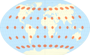 The Winkel tripel projection with Tissot's indicatrix of deformation
Consider a small circle on the surface of the Earth centred at a point P at latitude ϕ and longitude λ. Since the point scale varies with position and direction the projection of the circle on the projection will be distorted. Tissot proved that, as long as the distortion is not too great, the circle will become an ellipse on the projection. In general the dimension, shape and orientation of the ellipse will change over the projection. Superimposing these distortion ellipses on the map projection conveys the way in which the point scale is changing over the map. The distortion ellipse is known as Tissot's indicatrix. The example shown here is the Winkel tripel projection, the standard projection for world maps made by the National Geographic Society. The minimum distortion is on the central meridian at latitudes of 30 degrees (North and South). (Other examples[4][5]).
Point scale for normal cylindrical projections of the sphere

The key to a quantitative understanding of scale is to consider an infinitesimal element on the sphere. The figure shows a point P at latitude ϕ and longitude λ on the sphere. The point Q is at latitude φ + δφ and longitude λ + δλ. The lines PK and MQ are arcs of meridians of length aδφ where a is the radius of the sphere and ϕ is in radian measure. The lines PM and KQ are arcs of parallel circles of length (acos ϕ)δλ withλ in radian measure. In deriving a point property of the projection at P it suffices to take an infinitesimal element PMQK of the surface: in the limit of Q approaching P such an element tends to an infinitesimally small planar rectangle.
 Infinitesimal elements on the sphere and a normal cylindrical projection
Normal cylindrical projections of the sphere have x = aλ and y a function of latitude only. Therefore the infinitesimal element PMQK on the sphere projects to an infinitesimal element P'M'Q'K' which is an exact rectangle with a base δx = aδλ and height δy. By comparing the elements on sphere and projection we can immediately deduce expressions for the scale factors on parallels and meridians. (We defer the treatment of the scale in a general direction to a mathematical addendum to this page.)
-
- parallel scale factor

- meridian scale factor

- parallel scale factor
Note that the parallel scale factor k = sec ϕ is independent of the definition of y(ϕ) so it is the same for all normal cylindrical projections. It is useful to note that
-
- at latitude 30 degrees the parallel scale is

- at latitude 45 degrees the parallel scale is

- at latitude 60 degrees the parallel scale is

- at latitude 80 degrees the parallel scale is

- at latitude 85 degrees the parallel scale is

- at latitude 30 degrees the parallel scale is
The following examples illustrate three normal cylindrical projections and in each case the variation of scale with position and direction is illustrated by the use of Tissot's indicatrix.
Three examples of normal cylindrical projection
The equirectangular projection
 The equidistant projection with Tissot's indicatrix of deformation
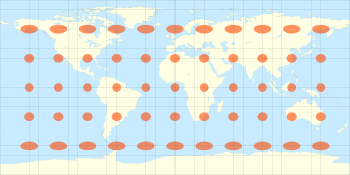
The equirectangular projection,[1][2][3] also known as the Plate Carrée (French for "flat square") or (somewhat misleadingly) the equidistant projection, is defined by
- x = aλ, y = aϕ,
where a is the radius of the sphere, λ is the longitude from the central meridian of the projection (here taken as the Greenwich meridian at λ = 0) and ϕ is the latitude. Note that λ and ϕ are in radians (obtained by multiplying the degree measure by a factor of π/180). The longitude λ is in the range [ − π,π] and the latitude ϕ is in the range [ − π / 2,π / 2].
Since y'(ϕ) = 1 the previous section gives
- parallel scale, meridian scale

For the calculation of the point scale in an arbitrary direction see addendum.
The figure illustrates the Tissot indicatrix for this projection. On the equator h=k=1 and the circular elements are undistorted on projection. At higher latitudes the circles are distorted into an ellipse given by stretching in the parallel direction only: there is no distortion in the meridian direction. The ratio of the major axis to the minor axis is sec ϕ. Clearly the area of the ellipse increases by the same factor.
It is instructive to consider the use of bar scales that might appear on a printed version of this projection. The scale is true (k=1) on the equator so that multiplying its length on a printed map by the inverse of the RF (or principal scale) gives the actual circumference of the Earth. The bar scale on the map is also drawn at the true scale so that transferring a separation between two points on the equator to the bar scale will give the correct distance between those points. The same is true on the meridians. On a parallel other than the equator the scale is sec ϕ so when we transfer a separation from a parallel to the bar scale we must divide the bar scale distance by this factor to obtain the distance between the points when measured along the parallel (which is not the true distance along a great circle). On a line at a bearing of say 45 degrees (
 ) the scale is continuously varying with latitude and transferring a separation along the line to the bar scale does not give a distance related to the true distance in any simple way. (But see addendum). Even if we could work out a distance along this line of constant bearing its relevance is questionable since such a line on the projection corresponds to a complicated curve on the sphere. For these reasons bar scales on small scale maps must be used with extreme caution.
Mercator projection
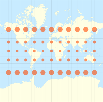 The Mercator projection with Tissot's indicatrix of deformation. (The distortion increases without limit at higher latitudes)
The Mercator projection maps the sphere to a rectangle (of infinite extent in the y-direction) by the equations[1][2][3]
where a,
 and
and  are as in the previous example. Since y'(ϕ) = asec ϕ the scale factors are:
parallel scale
meridian scale
In the mathematical addendum below we prove that the point scale in an arbitrary direction is also equal to sec ϕ so the scale is isotropic (same in all directions), its magnitude increasing with latitude as sec ϕ. In the Tissot diagram each infinitesimal circular element preserves its shape but is enlarged more and more as the latitude increases.
Lambert's equal area projection
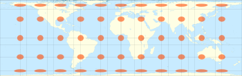 Lambert's normal cylindrical equal-area projection with Tissot's indicatrix of deformation
Lambert's equal area projection maps the sphere to a finite rectangle by the equations[1][2][3]
where a, λ and ϕ are as in the previous example. Since y'(ϕ) = cos ϕ the scale factors are
- parallel scale
- meridian scale

The calculation of the point scale in an arbitrary direction is given below.
The vertical and horizontal scales now compensate each other (hk=1) and in the Tissot diagram each infinitesimal circular element is distorted into an ellipse of the same area as the undistorted circles on the equator.
Graphs of scale factors
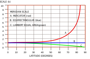
The graph shows the variation of the scale factors for the above three examples. The top plot shows the isotropic Mercator scale function: the scale on the parallel is the same as the scale on the meridian. The other plots show the meridian scale factor for the Equirectangular projection (h=1) and for the Lambert equal area projection. These last two projections have a parallel scale identical to that of the Mercator plot. For the Lambert note that the parallel scale (as Mercator A) increases with latitude and the meridian scale (C) decreases with latitude in such a way that hk=1, guaranteeing area conservation.
Scale variation on the Mercator projection
The Mercator point scale is unity on the equator because it is such that the auxiliary cylinder used in its construction is tangential to the Earth at the equator. For this reason the usual projection should be called a tangent projection. The scale varies with latitude as k = sec ϕ. Since sec ϕ tends to infinity as we approach the poles the Mercator map is grossly distorted at high latitudes and for this reason the projection is totally inappropriate for world maps (unless we are discussing navigation and rhumb lines). However, at a latitude of about 25 degrees the value of sec ϕ is about 1.1 so Mercator is accurate to within 10% in a strip of width 50 degrees centred on the equator. Narrower strips are better: a strip of width 16 degrees (centred on the equator) is accurate to within 1% or 1 part in 100.
A standard criterion for good large scale maps is that the accuracy should be within 4 parts in 10,000, or 0.04%, corresponding to k = 1.0004. Since sec ϕ attains this value at ϕ = 1.62 degrees (see figure below, red line). Therefore the tangent Mercator projection is highly accurate within a strip of width 3.24 degrees centred on the equator. This corresponds to north-south distance of about 360 km (220 mi). Within this strip Mercator is very good, highly accurate and shape preserving because it is conformal (angle preserving). These observations prompted the development of the transverse Mercator projections in which a meridian is treated 'like an equator' of the projection so that we obtain an accurate map within a narrow distance of that meridian. Such maps are good for countries aligned nearly north-south (like Great Britain) and a set of 60 such maps is used for the Universal Transverse Mercator (UTM). Note that in both these projections (which are based on various ellipsoids) the transformation equations for x and y and the expression for the scale factor are complicated functions of both latitude and longitude.
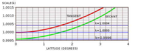 Scale variation near the equator for the tangent (red) and secant (green) Mercator projections.
Secant, or modified, projections
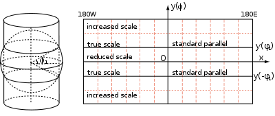
The basic idea of a secant projection is that the sphere is projected to a cylinder which intersects the sphere at two parallels, say ϕ1 north and south. Clearly the scale is now true at these latitudes whereas parallels beneath these latitudes are contracted by the projection and their (parallel) scale factor must be less than one. The result is that deviation of the scale from unity is reduced over a wider range of latitudes.
As an example, one possible secant Mercator projection is defined by
The numeric multipliers do not alter the shape of the projection but it does mean that the scale factors are modified:
-
-
- secant Mercator scale,

- secant Mercator scale,
-
Thus
- the scale on the equator is 0.9996,
- the scale is k=1 at a latitude given by ϕ1 where sec ϕ1 = 1 / 0.9996 = 1.00004 so that ϕ1 = 1.62 degrees,
- k=1.0004 at a latitude ϕ2 given by sec ϕ2 = 1.0004 / 0.9996 = 1.0008 for which ϕ2 = 2.29 degrees. Therefore the projection has 1 < k < 1.0004 , that is an accuracy of 0.04%, over a wider strip of 4.58 degrees (compared with 3.24 degrees for the tangent form).
This is illustrated by the lower (green) curve in the figure of the previous section.
Such narrow zones of high accuracy are used in the UTM and the British OSGB projection, both of which are secant, transverse Mercator on the ellipsoid with the scale on the central meridian constant at k0 = 0.9996. The isoscale lines with k = 1 are slightly curved lines approximately 180 km east and west of the central meridian. The maximum value of the scale factor is 1.001 for UTM and 1.0007 for OSGB.
The lines of unit scale at latitude ϕ1 (north and south), where the cylindrical projection surface intersects the sphere, are the standard parallels of the secant projection.
Whilst a narrow band with | k − 1 | < 0.0004 is important for high accuracy mapping at a large scale, for world maps much wider spaced standard parallels are used to control the scale variation. Examples are
- Behrmann with standard parallels at 30N, 30S.
- Gall equal area with standard parallels at 45N, 45S.
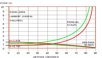 Scale variation for the Lambert (green) and Gall (red) equal area projections.
The scale plots for the latter are shown below compared with the Lambert equal area scale factors. In the latter the equator is a single standard parallel and the parallel scale increases from k=1 to compensate the decrease in the meridian scale. For the Gall the parallel scale is reduced at the equator (to k=0.707) whilst the meridian scale is increased (to k=1.414). This gives rise to the gross distortion of shape in the Gall-Peters projection. (On the globe Africa is about as long as it is broad). Note that the meridian and parallel scales are both unity on the standard parallels.
Mathematical addendum
Infinitesimal elements on the sphere and a normal cylindrical projectionFor normal cylindrical projections the geometry of the infinitesimal elements gives
The relationship between the angles β and α is
For the Mercator projection y'(ϕ) = asec ϕ giving α = β: angles are preserved. (Hardly surprising since this is the relation used to derive Mercator). For the equidistant and Lambert projections we have y'(ϕ) = a and y'(ϕ) = acos ϕ respectively so the relationship between α and β depends upon the latitude ϕ. Denote the point scale at P when the infinitesimal element PQ makes an angle
 with the meridian by μα. It is given by the ratio of distances:
Setting δx = aδλ and substituting δϕ and δy from equations (a) and (b) respectively gives
For the projections other than Mercator we must first calculate β from α and ϕ using equation (c), before we can find μα. For example the equirectangular projection has y' = a so that
If we consider a line of constant slope β on the projection both the corresponding value of α and the scale factor along the line are complicated functions of ϕ. There is no simple way of transferring a general finite separation to a bar scale and obtaining meaningful results.
References
- ^ a b c d e Snyder, John P. (1987). Map Projections - A Working Manual. U.S. Geological Survey Professional Paper 1395. United States Government Printing Office, Washington, D.C..This paper can be downloaded from USGS pages. It gives full details of most projections, together with introductory sections, but it does not derive any of the projections from first principles. Derivation of all the formulae for the Mercator projections may be found in The Mercator Projections.
- ^ a b c d Flattening the Earth: Two Thousand Years of Map Projections, John P. Snyder, 1993, pp. 5-8, ISBN 0-226-76747-7. This is a survey of virtually all known projections from antiquity to 1993.
- ^ a b c d The Mercator Projections A pedagogical derivation of the formulae describing many of the variants of the Mercator projections. In particular normal and transverse projections on the sphere and ellipsoid along with their modified versions. It concludes with the Redfearn formulae used for the Transverse Mercator on the ellipsoid.
- ^ Examples of Tissot's indicatrix. Some beautiful illustrations of the Tissot Indicatrix applied to a variety of projections other than normal cylindrical.
- ^ Further examples of Tissot's indicatrix at Wikipedia commons.
Categories: -


![y = a\ln \left[\tan \left(\frac{\pi}{4} + \frac{\phi}{2} \right) \right]](2/4c287e340e4121483852e4241042de4e.png)


![\mu_\alpha(\phi) = \sec\phi \left[\frac{\sin\alpha}{\sin\beta}\right].](3/bb3778d9000d31c2a7a1d022d4f3cdfe.png)

Wikimedia Foundation. 2010.