- Noncentral hypergeometric distributions
-
In statistics, the hypergeometric distribution is the discrete probability distribution generated by picking colored balls at random from an urn without replacement.
Various generalizations to this distribution exist for cases where the picking of colored balls is biased so that balls of one color are more likely to be picked than balls of another color.
This can be illustrated by the following example. Assume that an opinion poll is conducted by calling random telephone numbers. Unemployed people are more likely to be home and answer the phone than employed people are. Therefore, unemployed respondents are likely to be over-represented in the sample. The probability distribution of employed versus unemployed respondents in a sample of n respondents can be described as a noncentral hypergeometric distribution.
The description of biased urn models is complicated by the fact that there is more than one noncentral hypergeometric distribution. Which distribution you get depends on whether items (e.g. colored balls) are sampled one by one in a manner where there is competition between the items, or they are sampled independently of each other.
There is widespread confusion about this fact. The name noncentral hypergeometric distribution has been used for two different distributions, and several scientists have used the wrong distribution or erroneously believed that the two distributions were identical.
The use of the same name for two different distributions has been possible because these two distributions were studied by two different groups of scientists with hardly any contact with each other.
Agner Fog (2007, 2008) has suggested that the best way to avoid confusion is to use the name Wallenius' noncentral hypergeometric distribution for the distribution of a biased urn model where a predetermined number of items are drawn one by one in a competitive manner, while the name Fisher's noncentral hypergeometric distribution is used where items are drawn independently of each other, so that the total number of items drawn is known only after the experiment. The names refer to Kenneth Ted Wallenius and R. A. Fisher who were the first to describe the respective distributions.
Fisher's noncentral hypergeometric distribution has previously been given the name extended hypergeometric distribution, but this name is rarely used in the scientific literature, except in handbooks that need to distinguish between the two distributions. Some scientists are strongly opposed to using this name.
A thorough explanation of the difference between the two noncentral hypergeometric distributions is obviously needed here.
Contents
Wallenius' noncentral hypergeometric distribution
Main article: Wallenius' noncentral hypergeometric distributionWallenius' distribution can be explained as follows. Assume that an urn contains m1 red balls and m2 white balls, totalling N = m1 + m2 balls. n balls are drawn at random from the urn one by one without replacement. Each red ball has the weight ω1, and each white ball has the weight ω2. We assume that the probability of taking a particular ball is proportional to its weight. The physical property that determines the odds may be something else than weight, such as size or slipperiness or whatever, but it is convenient to use the word weight for the odds parameter.
The probability that the first ball picked is red is equal to the weight fraction of red balls:
The probability that the second ball picked is red depends on whether the first ball was red or white. If the first ball was red then the above formula is used with m1 reduced by one. If the first ball was white then the above formula is used with m2 reduced by one.
The important fact that distinguishes Wallenius' distribution is that there is competition between the balls. The probability that a particular ball is taken in a particular draw depends not only on its own weight, but also on the total weight of the competing balls that remain in the urn at that moment. And the weight of the competing balls depends on the outcomes of all preceding draws.
A multivariate version of Wallenius' distribution is used if there are more than two different colors.
The distribution of the balls that are not drawn is a complementary Wallenius' noncentral hypergeometric distribution.
Fisher's noncentral hypergeometric distribution
Main article: Fisher's noncentral hypergeometric distributionIn the Fisher model, the fates of the balls are independent and there is no dependence between draws. We may as well take all n balls at the same time. Each ball has no "knowledge" of what happens to the other balls. For the same reason, it is impossible to know the value of n before the experiment. If we tried to fix the value of n then we would have no way of preventing ball number n+1 from being taken without violating the principle of independence between balls. n is therefore a random variable, and the Fisher distribution is a conditional distribution which can only be determined after the experiment when n is known. The unconditional distribution is two independent binomials, one for each color.
Fisher's distribution can simply be defined as the conditional distribution of two or more independent binomial variates dependent upon their sum. A multivariate version of the Fisher's distribution is used if there are more than two colors of balls.
The difference between the two noncentral hypergeometric distributions
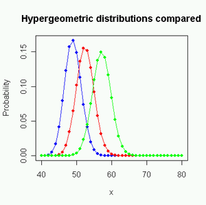 Comparison of distributions with same odds:
Blue: Wallenius ω=0.5
Red: Fisher ω=0.5
Green: Central hypergeometric ω=1.
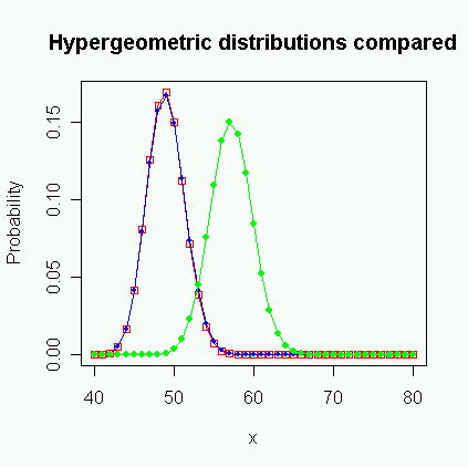
m1=80, m2=60, n=100 Comparison of distributions with same mean:
Blue: Wallenius ω=0.5
Red: Fisher ω=0.28
Green: Central hypergeometric ω=1.
m1=80, m2=60, n=100
Wallenius’ and Fisher’s distributions are approximately equal when the odds ratio ω = ω1 / ω2 is near 1, and n is low compared to the total number of balls, N. The difference between the two distributions becomes higher when the odds ratio is far from one and n is near N. The two distributions approximate each other better when they have the same mean than when they have the same odds (see figures above).Both distributions degenerate into the hypergeometric distribution when the odds ratio is 1, or to the binomial distribution when n = 1.
To understand why the two distributions are different, we may consider the following extreme example: An urn contains one red ball with the weight 1000, and a thousand white balls each with the weight 1. We want to calculate the probability that the red ball is not taken.
First we consider the Wallenius model. The probability that the red ball is not taken in the first draw is 1000/2000 = ½. The probability that the red ball is not taken in the second draw, under the condition that it was not taken in the first draw, is 999/1999 ≈ ½. The probability that the red ball is not taken in the third draw, under the condition that it was not taken in the first two draws, is 998/1998 ≈ ½. Continuing in this way, we can calculate that the probability of not taking the red ball in n draws is approximately 2−n as long as n is small compared to N. In other words, the probability of not taking a very heavy ball in n draws falls almost exponentially with n in Wallenius’ model. The exponential function arises because the probabilities for each draw are all multiplied together.
This is not the case in Fisher’s model where balls are taken independently, and possibly simultaneously. Here the draws are independent and the probabilities are therefore not multiplied together. The probability of not taking the heavy red ball in Fisher’s model is approximately 1/(n+1). The two distributions are therefore very different in this extreme case, even though they are quite similar in less extreme cases.
The following conditions must be fulfilled for Wallenius’ distribution to be applicable:
- Items are taken randomly from a finite source containing different kinds of items without replacement.
- Items are drawn one by one.
- The probability of taking a particular item at a particular draw is equal to its fraction of the total "weight" of all items that have not yet been taken at that moment. The weight of an item depends only on its kind (color).
- The total number n of items to take is fixed and independent of which items happen to be taken first.
The following conditions must be fulfilled for Fisher’s distribution to be applicable:
- Items are taken randomly from a finite source containing different kinds of items without replacement.
- Items are taken independently of each other. Whether one item is taken is independent of whether another item is taken. Whether one item is taken before, after, or simultaneously with another item is irrelevant.
- The probability of taking a particular item is proportional to its "weight". The weight of an item depends only on its kind (color).
- The total number n of items that will be taken is not known before the experiment.
- n is determined after the experiment and the conditional distribution for n known is desired.
Examples
The following examples will further clarify which distribution to use in different situations.
Example 1
You are catching fish in a small lake that contains a limited number of fish. There are different kinds of fish with different weights. The probability of catching a particular fish at a particular moment is proportional to its weight.
You are catching the fish one by one with a fishing rod. You have decided to catch n fish. You are determined to catch exactly n fish regardless of how long time it may take. You are stopping after you have caught n fish even if you can see more fish that are tempting you.
This scenario will give a distribution of the types of fish caught that is equal to Wallenius’ noncentral hypergeometric distribution.
Example 2
You are catching fish as in example 1, but you are using a big net. You are setting up the net one day and coming back the next day to remove the net. You count how many fish you have caught and then you go home regardless of how many fish you have caught. Each fish has a probability of getting into the net that is proportional to its weight but independent of what happens to the other fish.
The total number of fish that will be caught in this scenario is not known in advance. The expected number of fish caught is therefore described by multiple binomial distributions, one for each kind of fish.
After the fish have been counted, the total number n of fish is known. The probability distribution when n is known (but the number of each type is not known yet) is Fisher’s noncentral hypergeometric distribution.
Example 3
You are catching fish with a small net. It is possible that more than one fish can go into the net at the same time. You are using the net multiple times until you have got at least n fish.
This scenario gives a distribution that lies between Wallenius’ and Fisher’s distributions. The total number of fish caught can vary if you are getting too many fish in the last catch. You may put the excess fish back into the lake, but this still doesn’t give Wallenius’ distribution. This is because you are catching multiple fish at the same time. The condition that each catch depends on all previous catches does not hold for fish that are caught simultaneously or in the same operation.
The resulting distribution will be close to Wallenius’ distribution if there are only few fish in the net in each catch and you are catching many times. The resulting distribution will be close to Fisher’s distribution if there are many fish in the net in each catch and you are catching few times.
Example 4
You are catching fish with a big net. Fish are swimming into the net randomly in a situation that resembles a Poisson process. You are watching the net all the time and take up the net as soon as you have caught exactly n fish.
The resulting distribution will be close to Fisher’s distribution because the fish swim into the net independently of each other. But the fates of the fish are not totally independent because a particular fish can be saved from getting caught if n other fish happen to get into the net before the time that this particular fish would have been caught. This is more likely to happen if the other fish are heavy than if they are light.
Example 5
You are catching fish one by one with a fishing rod as in example 1. You need a particular amount of fish in order to feed your family. You are stopping when the total weight of the fish you have caught exceeds a predetermined limit. The resulting distribution will be close to Wallenius’ distribution, but not exactly because the decision to stop depends on the weight of the fish you have caught so far. n is therefore not known exactly before the fishing trip.
Conclusion to the examples
These examples show that the distribution of the types of fish you catch depends on the way they are caught. Many situations will give a distribution that lies somewhere between Wallenius’ and Fisher’s noncentral hypergeometric distributions.
An interesting consequence of the difference between these two distributions is that you will get more of the heavy fish, on average, if you catch n fish one by one than if you catch all n at the same time.
These conclusions can of course be applied to biased sampling of other items than fish. In general, we can say that the odds parameter has a stronger effect in Wallenius' distribution than in Fisher's distribution, especially when n/N is high.
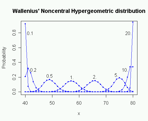
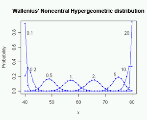 Probability mass function for Wallenius' Noncentral Hypergeometric Distribution for different values of the odds ratio ω.
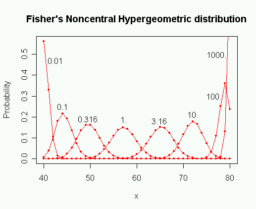
m1 = 80, m2 = 60, n = 100, ω = 0.1 ... 20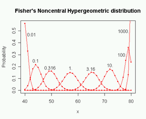 Probability mass function for Fisher's Noncentral Hypergeometric Distribution for different values of the odds ratio ω.
m1 = 80, m2 = 60, n = 100, ω = 0.01 ... 1000See also
- Wallenius' noncentral hypergeometric distribution
- Fisher's noncentral hypergeometric distribution
- hypergeometric distribution
- urn problem
- Bias
- Biased sample
References
Johnson, N. L.; Kemp, A. W.; Kotz, S. (2005), Univariate Discrete Distributions, Hoboken, New Jersey: Wiley and Sons.
McCullagh, P.; Nelder, J. A. (1983), Generalized Linear Models, London: Chapman and Hall.
Fog, Agner (2007), Random number theory, http://www.agner.org/random/theory/.
Fog, Agner (2008), "Calculation Methods for Wallenius' Noncentral Hypergeometric Distribution", Communications in statictics, Simulation and Computation 37 (2): 258–273, doi:10.1080/03610910701790269.
Categories:- Discrete distributions


Wikimedia Foundation. 2010.