Competitive Lotka–Volterra equations

The competitive Lotka–Volterra equations are a simple model of the population dynamics of species competing for some common resource. They can be further generalised to include trophic interactions.

Overview

The form is similar to the Lotka–Volterra equations for predation in that the equation for each species has one term for self-interaction and one term for the interaction with other species. In the equations for predation, the base population model is exponential. For the competition equations, the logistic equation is the basis.

The logistic population model, when used by ecologists often takes the following form:

${dx \over dt} = rx\left(1-{x \over K}\right).$

Here x is the size of the population at a given time, r is inherent per-capita growth rate, and K is the carrying capacity.

Two species

Given two populations, x₁ and x₂, with logistic dynamics, the Lotka–Volterra formulation adds an additional term to account for the species' interactions. Thus the competitive Lotka–Volterra equations are:

${dx_1 \over dt} = r_1x_1\left(1-\left({x_1+\alpha_{12}x_2 \over K_1}\right) \right)$

${dx_2 \over dt} = r_2x_2\left(1-\left({x_2+\alpha_{21}x_1 \over K_2}\right) \right).$

Here, α₁₂ represents the effect species 2 has on the population of species 1 and α₂₁ represents the effect species 1 has on the population of species 2. These values do not have to be equal. Because this is the competitive version of the model, all interactions must be harmful (competition) and therefore all α-values are positive. Also, note that each species can have its own growth rate and carrying capacity.

N species

This model can be generalized to any number of species competing against each other. One can think of the populations and growth rates as vectors and the interaction α's as a matrix. Then the equation for any species i becomes

$\frac{dx_i}{dt} = r_i x_i \left(1- \frac{\sum_{j=1}^N \alpha_{ij}x_j}{K_i} \right)$

or, if the carrying capacity is pulled into the interaction matrix (this doesn't actually change the equations, only how the interaction matrix is defined),

$\frac{dx_i}{dt} = r_i x_i \left( 1 - \sum_{j=1}^N \alpha_{ij}x_j \right)$

where N is the total number of interacting species. For simplicity all self-interacting terms α_ii are often set to 1.

Possible dynamics

The definition of a competitive Lotka-Volterra system assumes that all values in the interaction matrix are positive or 0 (α_ij ≥ 0 for all i,j). If it is also assumed that the population of any species will increase in the absence of competition unless the population is already at the carrying capacity (r_i > 0 for all i), then some definite statements can be made about the behavior of the system.

1. The populations of all species will be bounded between 0 and 1 at all times (0 ≤ x_i ≤ 1, for all i) as long as the populations started out positive.
2. Smale^[1] showed that Lotka-Volterra systems that meet the above conditions and have five or more species (N ≥ 5) can exhibit any asymptotic behavior, including a fixed point, a limit-cycle, an n-torus, or attractors.
3. Hirsch^[2][3][4] proved that all of the dynamics of the attractor occur on a manifold of dimension N-1. This basically says that the attractor cannot have dimension greater than N-1. Why is this important? A limit-cycle cannot exist in fewer than two dimensions. A n-torus cannot exist in less than n dimensions, and finally, chaos cannot occur in less than three dimensions. So, Hirsch proved that competitive Lotka–Volterra systems cannot exhibit a limit-cycle for N < 3, or any torus or chaos for N < 4. This is still in agreement with Smale that any dynamics can occur for N ≥ 5.
   • More specifically, Hirsch showed there is an invariant set C that is homeomorphic to the (N-1)-dimensional simplex
     $\Delta_{N-1} = \left \{ x_i : x_i \ge 0, \sum x_i = 1 \right \}$
     and is a global attractor of every point excluding the origin. This carrying simplex contains all of the asymptotic dynamics of the system.
4. To create a stable ecosystem the α_ij matrix must have all positive eigenvalues. For large N systems Lotka-Volterra models are either unstable or have low connectivity. Kondoh ^[5] and Ackland and Gallagher ^[6] have independently shown that large, stable Lotka-Volterra systems arise if the elements of α_ij (i.e. the features of the species) can evolve in accordance with natural selection.

4-dimensional example

The competitive Lotka–Volterra system plotted in phase space with the x₄ value represented by the color.

A simple 4-Dimensional example of a competitive Lotka–Volterra system has been characterized by Vano et al.^[7] Here the growth rates and interaction matrix have been set to

$r_i = \begin{bmatrix} 1 \\ 0.72 \\ 1.53 \\ 1.27 \end{bmatrix} \quad \alpha_{ij} = \begin{bmatrix} 1 & 1.09 & 1.52 & 0 \\ 0 & 1 & 0.44 & 1.36 \\ 2.33 & 0 & 1 & 0.47 \\ 1.21 & 0.51 & 0.35 & 1 \end{bmatrix}.$

This system is chaotic and has a largest Lyapunov exponent of 0.0203. From the theorems by Hirsch, it is one of the lowest dimensional chaotic competitive Lotka–Volterra systems. The Kaplan–Yorke dimension, a measure of the dimensionality of the attractor, is 2.074. This value is not a whole number, indicative of the fractal structure inherent in a strange attractor. The coexisting equilibrium point, the point at which all derivatives are equal to zero but that is not the origin, can be found by inverting the interaction matrix and multiplying by the unit column vector, and is equal to

$\overline{x} = \left ( \alpha_{ij} \right )^{-1} \begin{bmatrix} 1 \\ 1 \\ 1 \\ 1 \end{bmatrix} = \begin{bmatrix} 0.3013 \\ 0.4586 \\ 0.1307 \\ 0.3557 \end{bmatrix}.$

Note that there are always 2^N equilibrium points, but all others have at least one species' population equal to zero.

The eigenvalues of the system at this point are 0.0414±0.1903i, -0.3342, and -1.0319. This point is unstable due to the positive value of the real part of the complex eigenvalue pair. If the real part were negative, this point would be stable and the orbit would attract asymptotically. The transition between these two states, where the real part of the complex eigenvalue pair is equal to zero, is called a Hopf bifurcation.

Spatial arrangements

An illustration of spatial structure in nature. The strength of the interaction between bee colonies is a function of their proximity. Colonies A and B interact, as do colonies B and C. A and C do not interact directly, but affect each other through colony B.

Background

There are many situations where the strength of species' interactions depends on the physical distance of separation. Imagine bee colonies in a field. They will compete for food strongly with the colonies located near to them, weakly with further colonies, and not at all with colonies that are far away. This doesn't mean, however, that those far colonies can be ignored. There is a transitive effect that permeates through the system. If colony A interacts with colony B, and B with C, then C affects A through B. Therefore, if the competitive Lotka–Volterra equations are to be used for modeling such a system, they must incorporate this spatial structure.

Matrix organization

One possible way to incorporate this spatial structure is to modify the nature of the Lotka–Volterra equations to something like a reaction-diffusion system. It is much easier, however, to keep the format of the equations the same and instead modify the interaction matrix. For simplicity, consider a five species example where all of the species are aligned on a circle, and each interacts only with the two neighbors on either side with strength α_-1 and α₁ respectively. Thus, species 3 interacts only with species 2 and 4, species 1 interacts only with species 2 and 6, etc. The interaction matrix will now be

$\alpha_{ij} = \begin{bmatrix}1 & \alpha_1 & 0 & 0 & \alpha_{-1} \\ \alpha_{-1} & 1 & \alpha_1 & 0 & 0 \\ 0 & \alpha_{-1} & 1 & \alpha_1 & 0 \\ 0 & 0 & \alpha_{-1} & 1 & \alpha_1 \\ \alpha_1 & 0 & 0 & \alpha_{-1} & 1 \end{bmatrix}.$

If each species is identical in its interactions with neighboring species, then each row of the matrix is just a permutation of the first row. A simple, but non-realistic, example of this type of system has been characterized by Sprott et al.^[8] The coexisting equilibrium point for these systems has a very simple form given by the inverse of the sum of the row

$\overline{x}_i = \frac{1}{\sum_{j=1}^N \alpha_{ij}} = \frac{1}{\alpha_{-1} + 1 + \alpha_1}.$

Lyapunov functions

A Lyapunov function is a function of the system f = f(x) whose existence in a system demonstrates stability. It is often useful to imagine a Lyapunov function as the energy of the system. If the derivative of the function is equal to zero for some orbit not including the equilibrium point, then that orbit is a stable attractor, but it must be either a limit-cycle or n-torus - but not a strange attractor (this is because the largest Lyapunov exponent of a limit-cycle and n-torus are zero while that of a strange attractor is positive). If the derivative is less than zero everywhere except the equilibrium point, then the equilibrium point is a stable fixed point attractor. When searching a dynamical system for non-fixed point attractors, the existence of a Lyapunov function can help eliminate regions of parameter space where these dynamics are impossible.

The spatial system introduced above has a Lyapunov function that has been explored by Wildenberg et al.^[9] If all species are identical in their spatial interactions, then the interaction matrix is circulant. The eigenvalues of a circulant matrix are given by^[10]

$\lambda_k = \sum_{j=0}^{N-1} c_j\gamma^{kj}$

for k = 0_N − 1 and where γ = e^{i2π / N} the Nth root of unity. Here c_j is the jth value in the first row of the circulant matrix.

The Lyapunov function exists if the real part of the eigenvalues are positive (Re(λ_k > 0 for k = 0, …, N/2). Consider the system where α_-2 = a, α_-1 = b, α₁ = c, and α₂ = d. The Lyapunov function exists if

$\operatorname{Re}(\lambda_k) = \operatorname{Re} \left ( 1+\alpha_{-2}e^{i2 \pi k(N-2)/N}+\alpha_{-1}e^{i2 \pi k(N-1)/N}+\alpha_1e^{i2 \pi k/N}+\alpha_2e^{i4 \pi k/N} \right )$ $= 1+(\alpha_{-2}+\alpha_2)\cos \left ( \frac{i4 \pi k}{N} \right ) + (\alpha_{-1}+\alpha_1)\cos \left ( \frac{i2 \pi k}{N} \right ) > 0$

for k = 0, … ,N − 1. Now, instead of having to integrate the system over thousands of time steps to see if any dynamics other than a fixed point attractor exist, one need only determine if the Lyapunov function exists (note: the absence of the Lyapunov function doesn't guarantee a limit-cycle, torus, or chaos).

Example: Let α₋₂ = 0.451, α₋₁ = 0.5, and α₂ = 0.237. If α₁ = 0.5 then all eigenvalues are negative and the only attractor is a fixed point. If α₁ = 0.852 then the real part of one of the complex eigenvalue pair becomes positive and there is a strange attractor. The disappearance of this Lyapunov function coincides with a Hopf bifurcation.

Line systems and eigenvalues

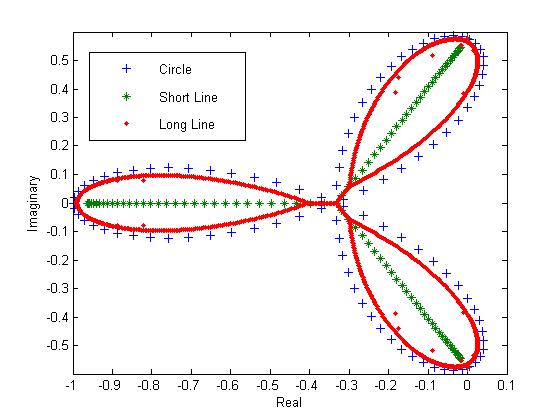
The eigenvalues of a circle, short line, and long line plotted in the complex plane

It is also possible to arrange the species into a line.^[9] The interaction matrix for this system is very similar to that of a circle except the interaction terms in the lower left and upper right of the matrix are deleted (those that describe the interactions between species 1 and N, etc.).

$\alpha_{ij} = \begin{bmatrix}1 & \alpha_1 & 0 & 0 & 0 \\ \alpha_{-1} & 1 & \alpha_1 & 0 & 0 \\ 0 & \alpha_{-1} & 1 & \alpha_1 & 0 \\ 0 & 0 & \alpha_{-1} & 1 & \alpha_1 \\ 0 & 0 & 0 & \alpha_{-1} & 1 \end{bmatrix}$

This change eliminates the Lyapunov function described above for the system on a circle, but most likely there are other Lyapunov functions that have not been discovered.

The eigenvalues of the circle system plotted in the complex plane form a trefoil shape. The eigenvalues from a short line form a sideways Y, but those of a long line begin to resemble the trefoil shape of the circle. This could be due to the fact that a long line is indistinguishable from a circle to those species far from the ends.

Cellular automata

A rule-based automaton model is equivalent to a Lotka–Volterra system and introduces 2D space, with either periodic or fixed boundaries.

Each site has three states, fox, bare, rabbit. Rules are as follows:

1. Pick a site (only stochastic updates allowed), and a neighbour.
2. If fox is adjacent to rabbit, rabbit gets eaten (becomes fox with probability r). Else fox dies with probability p.
3. If rabbit is adjacent to bare ground, reproduces with probability q.
4. If bare ground is adjacent to anything, the thing moves into bare ground.

These rules give a model like Lotka–Volterra, but the additional feature of a correlation length between regions oscillating differently. The correlation length is very long, and the model develops a wave structure.

Notes

1. ^ S. Smale, J. Math. Biol. 3, 5., 1976
2. ^ M. Hirsch, SIAM J. Math. Anal. 16, 423., 1985
3. ^ M. Hirsch, Nonlinearity 1, 51., 1988
4. ^ M. Hirsch, SIAM J. Math. Anal. 21, 1225., 1990
5. ^ Kondoh M Science 299, 1388 (2003)
6. ^ Ackland GJ and Gallagher ID Phys. Rev. Lett. 93, 158701 (2004)
7. ^ Vano, J.A., Wildenberg, J.C., Anderson, M.B., Noel, J.K., Sprott, J.C. Chaos in Low-Dimensional Lotka–Volterra Models of Competition. Submitted Nonlinearity. 2006
8. ^ Sprott, J.C., Wildenberg, J.C., Azizi, Y. A simple spatiotemporal chaotic Lotka–Volterra model. Chaos, Solitons & Fractals 26, 1035., 2005
9. ^ ^{a b} Wildenberg, J.C., Vano, J.A., Sprott, J.C. Complex spatiotemporal dynamics in Lotka–Volterra ring systems. Ecological Complexity 3, 140. 2006
10. ^ Hofbauer, J., Sigmund, K., 1988. The Theory of Evolution and Dynamical Systems. Cambridge University Press, Cambridge, U.K, p. 352.