- Discrete-time Fourier transform
-
In mathematics, the discrete-time Fourier transform (DTFT) is one of the specific forms of Fourier analysis. As such, it transforms one function into another, which is called the frequency domain representation, or simply the "DTFT", of the original function (which is often a function in the time-domain). But the DTFT requires an input function that is discrete. Such inputs are often created by digitally sampling a continuous function, like a person's voice.
The DTFT frequency-domain representation is always a periodic function. Since one period of the function contains all of the unique information, it is sometimes convenient to say that the DTFT is a transform to a "finite" frequency-domain (the length of one period), rather than to the entire real line.
Fourier transforms Continuous Fourier transform Fourier series Discrete Fourier transform Discrete-time Fourier transform Related transforms Contents
Definition
Given a discrete set of real or complex numbers:
![x[n], \; n\in\mathbb{Z}](7/5c7506e1fd33ac609168ae819788bd85.png) (integers), the discrete-time Fourier transform (or DTFT) of
(integers), the discrete-time Fourier transform (or DTFT) of ![x[n]\,](f/b0f955b87baf7377b98b47ed9c723949.png) is usually written:
is usually written:-
![X(\omega) = \sum_{n=-\infty}^{\infty} x[n] \,e^{-i \omega n}.](3/76369d772b8bb257c576b44f1aa05468.png)
(
Relationship to sampling
Often the
sequence represents the values (aka samples) of a continuous-time function,  , at discrete moments in time:
  , where
  is the sampling interval (in seconds), and
  is the sampling rate (samples per second). Then the DTFT provides an approximation of the continuous-time Fourier transform:
To understand this, consider the Poisson summation formula, which indicates that a periodic summation of function
 can be constructed from the samples of function
  The result is:
-
![X_{1/T}(f)\ \stackrel{\mathrm{def}}{=} \sum_{k=-\infty}^{\infty} X\left(f - k/T\right)
= \sum_{n=-\infty}^{\infty} \underbrace{T\cdot x(nT)}_{x[n]}\ e^{-i 2\pi f T n}](0/e103cc1cc0278a1d0366522ccf0a8259.png)
(
 comprises exact copies of that are shifted by multiples of ƒs and combined by addition. For sufficiently large ƒs, the k=0 term can be observed in the region [−ƒs/2, ƒs/2] with little or no distortion (aliasing) from the other terms.
With the following definition of a normalized frequency, the right-hand sides of Eq.2 and Eq.1 are identical:

Since
 represents ordinary frequency (cycles per second) and
  has units of samples per second, the units of
  are cycles per sample. It is common notational practice to replace this ratio with a single variable, called normalized frequency, which represents actual frequencies as multiples (usually fractional) of the sample rate.
  is also a normalized frequency, with units of radians per sample.
Periodicity
Sampling
causes its spectrum (DTFT) to become periodic. In terms of ordinary frequency, (cycles per second), the period is the sample rate, . In terms of normalized frequency, (cycles per sample), the period is 1. And in terms of (radians per sample), the period is 2π, which also follows directly from the periodicity of  . That is:
where both n and k are arbitrary integers. Therefore:
The popular alternate notation
 for the DTFT
  :
:- highlights the periodicity property, and
- helps distinguish between the DTFT and underlying Fourier transform of ; that is, (or ), and
- emphasizes the relationship of the DTFT to the Z-transform.
However, its relevance is obscured when the DTFT is formed by the frequency domain method (periodic summation), as discussed above. So the notation
is also commonly used, as in the table to follow.Inverse transform
The following inverse transforms recover the discrete-time sequence:
where
 is an integral over any interval of length λ. The integrals span one full period of the DTFT, which means that the x[n] samples are also the coefficients of a Fourier series expansion of the DTFT. Infinite limits of integration change the transform into an inverse [continuous-time] Fourier transform, which produces a sequence of Dirac impulses. That is:
Sampling the DTFT
A common practice is to compute an arbitrary number of samples (N) of one cycle of the periodic function X1 / T :
Since the kernel,
 is N-periodic, it can readily be shown that this is equivalent to the following discrete Fourier transform (DFT):
-
![X[k] = \sum_{N} x_N[n]\cdot e^{-i 2\pi \frac{kn}{N}},](2/ae2e6ea1eeb59bfbea5e908f2b4325a9.png)
(
where
 is a summation over any interval of length N, and
  is another periodic summation:
which is also the inverse DFT. In other words, our sampling of the DTFT causes the inverse transform to become periodic.
In order to evaluate Eq.3 numerically, we require a finite-length x[n] sequence. For instance, a long sequence might be truncated by a window function of length
 resulting in two cases worthy of special mention: L ≤ N and L = I•N, for some integer I (typically 6 or 8). For notational simplicity, consider the x[n] values below to represent the modified values.
When reduces to a summation of I blocks of length N. This goes by various names, such as multi-block windowing and window presum-DFT [1] [2] [3] . Multi-block window functions can provide excellent isolation (low spectral leakage) between the DTFT samples, which is usually a priority when implementing an FFT filter-bank (channelizer). With a conventional window function of length L, the DTFT would be undersampled (i.e. too much isolation), and important detail might be missed. But when the window function has a main lobe width on the order of length N, the resolutions of the sampling and the DTFT remain well-matched. Those kinds of windows are usually created using FIR filter design algorithms.
When the DFT is usually written in this more familiar form:
In order to take advantage of a fast Fourier transform algorithm for computing the DFT, the summation is usually performed over all N terms, even though N-L of them are zeros. Therefore, the case L < N is often referred to as zero-padding.
Spectral leakage, which increases as L decreases, is detrimental to certain important performance metrics, such as resolution of multiple frequency components and the amount of noise measured by each DTFT sample. But those things don't always matter, for instance when the x[n] sequence is a noiseless sinusoid (or a constant), shaped by a window function. Then it is a common practice to use zero-padding to graphically display and compare the detailed leakage patterns of window functions. To illustrate that for a rectangular window, consider the sequence:
![x[n] = e^{i 2\pi \frac{1}{8} n}](a/f6a529d964d547689fcfb0637143a30d.png) , and L = 64.
, and L = 64.
The two figures below are plots of the magnitude of two different sized DFTs, as indicated in their labels. In both cases, the dominant component is at the signal frequency:
 . Also visible on the right is the spectral leakage pattern of the L = 64 rectangular window. The illusion on the left is a result of sampling the DTFT at all of its zero-crossings. Rather than the DTFT of a finite-length sequence, it gives the impression of an infinitely long sinusoidal sequence. Contributing factors to the illusion are the use of a rectangular window, and the choice of a frequency (
 ) with exactly 8 (an integer) cycles per 64 samples.
 DFT for L = 64 and N = 64
 DFT for L = 64 and N = 256
Relationship to the Z-transform
The DTFT is a special case of the Z-transform. The bilateral Z-transform is defined as:
So the special case is:
 . Since
  , it is the evaluation of the Z-transform around the unit circle in the complex plane.
Table of discrete-time Fourier transforms
Some common transform pairs are shown below. The following notation applies:
 is an integer representing the discrete-time domain (in samples)
 is a real number in
  , representing continuous angular frequency (in radians per sample).
- The remainder of the transform
 is defined by:
- The remainder of the transform
![u[n] \!](f/b0fdbd85a77ceef12d141ef691eabb9e.png) is the discrete-time unit step function
is the discrete-time unit step function is the normalized sinc function
 is the Dirac delta function
![\delta [n] \!](f/12fc131638506475d9bb9f50bc3b42d5.png) is the Kronecker delta
is the Kronecker delta 
 is the rectangle function for arbitrary real-valued t:
 is the triangle function for arbitrary real-valued t:
Time domain
Frequency domain
Remarks 
![\delta [n - M] \!](b/cebeaaf3d6fd153519b2695b470d6888.png)

integer M ![\sum_{m = -\infty}^{\infty} \delta[n - M m] \!](a/87aedc1150118cf43e8e4032c8c41440.png)

integer M 
The 1 / (1 − e − iω) term must be interpreted as a distribution in the sense of a Cauchy principal value around its poles at ω = 2πk. ![a^{n} u[n]\!](b/60b8f6b97a0805ead19ac0aede09a335.png)

| a | < 1 

real number a 
![\pi \left[ \delta (\omega - a) + \delta (\omega + a) \right]](1/c71572b56a2c55584aca53d3d0087e23.png)
real number a 
![\frac{\pi}{i} \left[ \delta (\omega - a) - \delta ( \omega + a) \right]](4/394786f49727a8b7b0401964287fd4b0.png)
real number a ![\mathrm{rect} \left[ { ( n - M/2 ) \over M } \right]](4/a541ff492ffc8407bd3c86fe66cac8d7.png)
![{ \sin[ \omega (M+1) / 2 ] \over \sin( \omega / 2 ) } \, e^{ -i \omega M / 2 } \!](0/950296b2a9970d92f37ccc50b0a77938.png)
integer M ![\operatorname{sinc} [(a + n)]](d/42d0ce19eddbbb0d976fdf7829ae1e86.png)

real number a 

real number W


real numbers W


jω it works as a differentiator filter ![\frac{W}{(n + a)} \left\{ \cos [ \pi W (n+a)] - \operatorname{sinc} [ W (n+a)] \right\}](0/6a0d1751f486898561b37f060e3a6cf7.png)

real numbers W, a
![\frac{1}{\pi n^2} [(-1)^n - 1] \!](f/10f6b01347e817e0f3196f4305b2df45.png)


Hilbert transform ![\frac{C (A + B)}{2 \pi} \cdot \operatorname{sinc} \left[ \frac{A - B}{2\pi} n \right] \cdot \operatorname{sinc} \left[ \frac{A + B}{2\pi} n \right]](2/4b249fd22049eabe13c6e2ffb37d44ea.png)
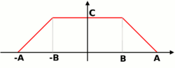
real numbers A, B
complex CProperties
This table shows some mathematical operations in the time-domain and the corresponding effects in the frequency domain.
 is the discrete convolution of two sequences
![x[n]^*\!](1/bb1ad27c1e964c58a894e0842c01d2a7.png) is the complex conjugate of
is the complex conjugate of ![x[n]\!](4/f04e9932b1bdccb47bb15c5ef53475c8.png)
Property Time domain Frequency domain 
Remarks Linearity ![a x[n] + b y[n] \!](5/4b56e446f69c22ab170df278170c46f9.png)

Shift in time ![x[n - k] \!](d/42db10711bdb344ce52c4b5d158fc80a.png)

integer k Shift in frequency (modulation) ![x[n]e^{ian} \!](c/e7cb66ead5d27230f042f546434d4de4.png)

real number a Time reversal ![x[- n] \!](0/a8069ffea484ccd085714ea675baa9c4.png)

Time conjugation 
Time reversal & conjugation ![x[-n]^* \!](d/61d36c43faf1a9c41e26b65f6ee40fe4.png)

Derivative in frequency ![\frac{n}{i} x[n] \!](6/cd681af35671ec47be7f064d527b0a3c.png)

Integral in frequency ![\frac{i}{n} x[n] \!](5/c05ecf25cb260110eb20b2e0955394c1.png)

Convolve in time ![x[n] * y[n] \!](8/5b8474366b0acdd770d83ed55c86ca59.png)

Multiply in time ![x[n] \cdot y[n] \!](3/1f36378f8b0b62c337ef19cee614fa32.png)

Periodic convolution Cross correlation ![\rho_{xy} [n] = x[-n]^* * y[n] \!](4/2846b8930d6d16572ff0b34b59f08fa5.png)

Parseval's theorem ![E = \sum_{n=-\infty}^{\infty} {x[n] \cdot y^*[n]} \!](a/00ad81cb23c5d6270ecdbebe53aa31b0.png)

Symmetry Properties
The Fourier Transform can be decomposed into a real and imaginary part or into an even and odd part.

or

Time Domain
Frequency Domain

![x^*[n]\!](2/c629e18c8a6821ac18eeeb8846dd57f9.png)

![x^*[-n]\!](1/3e1d724c56fc9874564ccd1f70b35d12.png)

Citations
- ^ Gumas, Charles Constantine (July 1997). "Window-presum FFT achieves high-dynamic range, resolution". Personal Engineering & Instrumentation News: 58–64.
- ^ Dahl, Jason F (2003). "Chapter 3.4". Time Aliasing Methods of Spectral Estimation (PhD thesis). Brigham Young University. http://contentdm.lib.byu.edu/ETD/image/etd157.pdf.
- ^ Lyons, Richard G. (June 2008). "DSP Tricks: Building a practical spectrum analyzer". EE Times. http://www.eetimes.com/design/embedded/4007611/DSP-Tricks-Building-a-practical-spectrum-analyzer.
References
- Alan V. Oppenheim and Ronald W. Schafer (1999). Discrete-Time Signal Processing (2nd Edition ed.). Prentice Hall Signal Processing Series. ISBN 0-13-754920-2.
- William McC. Siebert (1986). Circuits, Signals, and Systems. MIT Electrical Engineering and Computer Science Series. Cambridge, MA: MIT Press.
- Boaz Porat. A Course in Digital Signal Processing. John Wiley and Sons. pp. 27–29 and 104–105. ISBN 0-471-14961-6.
Digital signal processing Theory Sub-fields Techniques Discrete Fourier transform (DFT) · Discrete-time Fourier transform (DTFT) · Impulse invariance · bilinear transform · pole–zero mapping · Z-transform · advanced Z-transformSampling oversampling · undersampling · downsampling · upsampling · aliasing · anti-aliasing filter · sampling rate · Nyquist rate/frequencyCategories: -


![\begin{align}
\int_{-\infty}^\infty X_{1/T}(f)\cdot e^{i 2 \pi f t}\, df
&=\int_{-\infty}^\infty \left(\sum_{n=-\infty}^{\infty} T\cdot x(nT)\ e^{-i 2\pi f T n}\right)\cdot e^{i 2 \pi f t}\, df \\
&=\sum_{n=-\infty}^{\infty} T\cdot x(nT) \int_{-\infty}^\infty e^{-i 2\pi f T n}\cdot e^{i 2 \pi f t}\, df \\
&=\sum_{n=-\infty}^{\infty} x[n]\cdot \delta(t - n T).
\end{align}](4/f74a796883db9e3119339705dcfb2b89.png)
![\underbrace{X_{1/T}\left(\frac{k}{NT}\right)}_{X[k]} = \sum_{n=-\infty}^{\infty} x[n]\cdot e^{-i 2\pi \frac{kn}{N}} \quad \quad k = 0, \dots, N-1](6/e96d04e990834dde9564744b40d0ce7e.png)
![x_N[n]\ \stackrel{\text{def}}{=}\ \sum_{m=-\infty}^{\infty} x[n-mN],](f/07f6e2c29e01694061658716adcd93bb.png)
![X[k] = \sum_{n=0}^{N-1} x[n]\cdot e^{-i 2\pi \frac{kn}{N}}.](f/6af054543fca29ba09aab1bd885c7bb5.png)


![X(z) = \sum_{n=-\infty}^{\infty} x[n] \,z^{-n}](f/ebf4077bf748b204499cd73d8ce9312d.png)
![\mathrm{rect}(t) = \sqcap(t) = \begin{cases}
0 & \mbox{if } |t| > \frac{1}{2} \\[3pt]
\frac{1}{2} & \mbox{if } |t| = \frac{1}{2} \\[3pt]
1 & \mbox{if } |t| < \frac{1}{2}
\end{cases}](d/02dfb78ddb6c1f88b062ca0d076ef26f.png)


Wikimedia Foundation. 2010.