Curve fitting

"best fit" redirects here. For placing ("fitting") variable-sized objects in storage, see fragmentation (computer).

Curve fitting is the process of constructing a curve, or mathematical function, that has the best fit to a series of data points, possibly subject to constraints. Curve fitting can involve either interpolation, where an exact fit to the data is required, or smoothing, in which a "smooth" function is constructed that approximately fits the data. A related topic is regression analysis, which focuses more on questions of statistical inference such as how much uncertainty is present in a curve that is fit to data observed with random errors. Fitted curves can be used as an aid for data visualization, to infer values of a function where no data are available, and to summarize the relationships among two or more variables. Extrapolation refers to the use of a fitted curve beyond the range of the observed data, and is subject to a greater degree of uncertainty since it may reflect the method used to construct the curve as much as it reflects the observed data.

Different types of curve fitting

Fitting lines and polynomial curves to data points

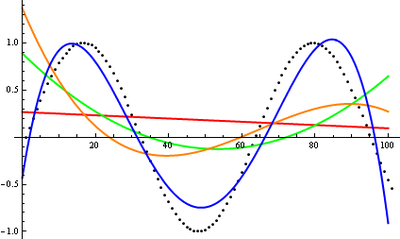Polynomial curves fitting points generated with a sine function.
Red line is a first degree polynomial, green line is second degree, orange line is third degree and blue is fourth degree

Let's start with a first degree polynomial equation:

$y = ax + b\;.$

This is a line with slope a. We know that a line will connect any two points. So, a first degree polynomial equation is an exact fit through any two points with distinct x coordinates.

If we increase the order of the equation to a second degree polynomial, we get:

$y = ax^2 + bx + c\;.$

This will exactly fit a simple curve to three points.

If we increase the order of the equation to a third degree polynomial, we get:

$y = ax^3 + bx^2 + cx + d\;.$

This will exactly fit four points.

A more general statement would be to say it will exactly fit four constraints. Each constraint can be a point, angle, or curvature (which is the reciprocal of the radius of an osculating circle). Angle and curvature constraints are most often added to the ends of a curve, and in such cases are called end conditions. Identical end conditions are frequently used to ensure a smooth transition between polynomial curves contained within a single spline. Higher-order constraints, such as "the change in the rate of curvature", could also be added. This, for example, would be useful in highway cloverleaf design to understand the rate of change of the forces applied to a car (see jerk), as it follows the cloverleaf, and to set reasonable speed limits, accordingly.

Bearing this in mind, the first degree polynomial equation could also be an exact fit for a single point and an angle while the third degree polynomial equation could also be an exact fit for two points, an angle constraint, and a curvature constraint. Many other combinations of constraints are possible for these and for higher order polynomial equations.

If we have more than n + 1 constraints (n being the degree of the polynomial), we can still run the polynomial curve through those constraints. An exact fit to all constraints is not certain (but might happen, for example, in the case of a first degree polynomial exactly fitting three collinear points). In general, however, some method is then needed to evaluate each approximation. The least squares method is one way to compare the deviations.

Now, you might wonder why we would ever want to get an approximate fit when we could just increase the degree of the polynomial equation and get an exact match. There are several reasons:

• Even if an exact match exists, it does not necessarily follow that we can find it. Depending on the algorithm used, we may encounter a divergent case, where the exact fit cannot be calculated, or it might take too much computer time to find the solution. Either way, you might end up having to accept an approximate solution.

• We may actually prefer the effect of averaging out questionable data points in a sample, rather than distorting the curve to fit them exactly.

• Runge's phenomenon: high order polynomials can be highly oscillatory. If we run a curve through two points A and B, we would expect the curve to run somewhat near the midpoint of A and B, as well. This may not happen with high-order polynomial curves, they may even have values that are very large in positive or negative magnitude. With low-order polynomials, the curve is more likely to fall near the midpoint (it's even guaranteed to exactly run through the midpoint on a first degree polynomial).

• Low-order polynomials tend to be smooth and high order polynomial curves tend to be "lumpy". To define this more precisely, the maximum number of ogee/inflection points possible in a polynomial curve is n-2, where n is the order of the polynomial equation. An inflection point is a location on the curve where it switches from a positive radius to negative. We can also say this is where it transitions from "holding water" to "shedding water". Note that it is only "possible" that high order polynomials will be lumpy, they could also be smooth, but there is no guarantee of this, unlike with low order polynomial curves. A fifteenth degree polynomial could have, at most, thirteen inflection points, but could also have twelve, eleven, or any number down to zero.

Now that we have talked about using a degree too low for an exact fit, let's also discuss what happens if the degree of the polynomial curve is higher than needed for an exact fit. This is bad for all the reasons listed previously for high order polynomials, but also leads to a case where there are an infinite number of solutions. For example, a first degree polynomial (a line) constrained by only a single point, instead of the usual two, would give us an infinite number of solutions. This brings up the problem of how to compare and choose just one solution, which can be a problem for software and for humans, as well. For this reason, it is usually best to choose as low a degree as possible for an exact match on all constraints, and perhaps an even lower degree, if an approximate fit is acceptable.

For more details, Polynomial interpolation.

Fitting other curves to data points

Other types of curves, such as conic sections (circular, elliptical, parabolic, and hyperbolic arcs) or trigonometric functions (such as sine and cosine), may also be used, in certain cases. For example, trajectories of objects under the influence of gravity follow a parabolic path, when air resistance is ignored. Hence, matching trajectory data points to a parabolic curve would make sense. Tides follow sinusoidal patterns, hence tidal data points should be matched to a sine wave, or the sum of two sine waves of different periods, if the effects of the Moon and Sun are both considered.

Algebraic fit versus geometric fit for curves

For algebraic analysis of data, "fitting" usually means trying to find the curve that minimizes the vertical (y-axis) displacement of a point from the curve (e.g., ordinary least squares). However for graphical and image applications geometric fitting seeks to provide the best visual fit; which usually means trying to minimize the orthogonal distance to the curve (e.g., total least squares), or to otherwise include both axes of displacement of a point from the curve. Geometric fits are not popular because they usually require non-linear and/or iterative calculations, although they have the advantage of a more aesthetic and geometrically accurate result.

Fitting a circle by geometric fit

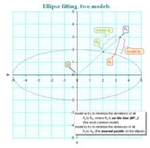different models of fitting

Coope^[1] approaches the problem of trying to find the best visual fit of circle to a set of 2D data points. The method elegantly transforms the ordinarily non-linear problem into a linear problem that can be solved without using iterative numerical methods, and is hence an order of magnitude faster than previous techniques.

Fitting an ellipse by geometric fit

The above technique is extended to general ellipses^[2] by adding a non-linear step, resulting in a method that is fast, yet finds visually pleasing ellipses of arbitrary orientation and displacement.

Application to surfaces

Note that while this discussion was in terms of 2D curves, much of this logic also extends to 3D surfaces, each patch of which is defined by a net of curves in two parametric directions, typically called u and v. A surface may be composed of one or more surface patches in each direction.

For more details, see the computer representation of surfaces article.

Software

Many statistical packages such as R and numerical software such as the GNU Scientific Library, SciPy and OpenOpt include commands for doing curve fitting in a variety of scenarios. There are also programs specifically written to do curve fitting; they can be found in the lists of statistical and numerical analysis programs as well as in Category:Regression and curve fitting software.

See also

• Levenberg–Marquardt algorithm
• Nonlinear regression
• Smoothing
• Total least squares
• Overfitting

References

1. ^ Coope, I.D., Circle fitting by linear and nonlinear least squares, Journal of Optimization Theory and Applications Volume 76, Issue 2, New York: Plenum Press, February 1993
2. ^ Paul Sheer, A software assistant for manual stereo photometrology, M.Sc. thesis, 1997

References

Wikimedia Foundation. 2010.