Calculus

This article is about the branch of mathematics. For other uses, see Calculus (disambiguation).

Topics in Calculus

Fundamental theorem Limits of functions Continuity Mean value theorem Differential calculus  Derivative Change of variables Implicit differentiation Taylor's theorem Related rates Rules and identities: Power rule, Product rule, Quotient rule, Chain rule Integral calculus  Integral Lists of integrals Improper integrals Integration by: parts, disks, cylindrical shells, substitution, trigonometric substitution, partial fractions, changing order Vector calculus  Gradient Divergence Curl Laplacian Gradient theorem Green's theorem Stokes' theorem Divergence theorem Multivariable calculus  Matrix calculus Partial derivative Multiple integral Line integral Surface integral Volume integral Jacobian

Calculus (Latin, calculus, a small stone used for counting) is a branch of mathematics focused on limits, functions, derivatives, integrals, and infinite series. This subject constitutes a major part of modern mathematics education. It has two major branches, differential calculus and integral calculus, which are related by the fundamental theorem of calculus. Calculus is the study of change,^[1] in the same way that geometry is the study of shape and algebra is the study of operations and their application to solving equations. A course in calculus is a gateway to other, more advanced courses in mathematics devoted to the study of functions and limits, broadly called mathematical analysis. Calculus has widespread applications in science, economics, and engineering and can solve many problems for which algebra alone is insufficient.

Historically, calculus was called "the calculus of infinitesimals", or "infinitesimal calculus". More generally, calculus (plural calculi) refers to any method or system of calculation guided by the symbolic manipulation of expressions. Some examples of other well-known calculi are propositional calculus, variational calculus, lambda calculus, pi calculus, and join calculus.

History

Main article: History of calculus

Ancient

Isaac Newton developed the use of calculus in his laws of motion and gravitation.

The ancient period introduced some of the ideas that led to integral calculus, but does not seem to have developed these ideas in a rigorous or systematic way. Calculations of volumes and areas, one goal of integral calculus, can be found in the Egyptian Moscow papyrus (c. 1820 BC), but the formulas are mere instructions, with no indication as to method, and some of them are wrong.^[2] From the age of Greek mathematics, Eudoxus (c. 408−355 BC) used the method of exhaustion, which prefigures the concept of the limit, to calculate areas and volumes, while Archimedes (c. 287−212 BC) developed this idea further, inventing heuristics which resemble the methods of integral calculus.^[3] The method of exhaustion was later reinvented in China by Liu Hui in the 3rd century AD in order to find the area of a circle.^[4] In the 5th century AD, Zu Chongzhi established a method which would later be called Cavalieri's principle to find the volume of a sphere.^[5]

Medieval

In the 14th Century Indian mathematician Madhava of Sangamagrama and the Kerala school of astronomy and mathematics stated many components of calculus such as the Taylor series, infinite series approximations, an integral test for convergence, early forms of differentiation, term by term integration, iterative methods for solutions of non-linear equations, and the theory that the area under a curve is its integral. Some consider the Yuktibhāṣā to be the first text on calculus.^[6]

Modern

"The calculus was the first achievement of modern mathematics and it is difficult to overestimate its importance. I think it defines more unequivocally than anything else the inception of modern mathematics, and the system of mathematical analysis, which is its logical development, still constitutes the greatest technical advance in exact thinking." —John von Neumann[7]

In Europe, the foundational work was a treatise due to Bonaventura Cavalieri, who argued that volumes and areas should be computed as the sums of the volumes and areas of infinitesimally thin cross-sections. The ideas were similar to Archimedes' in The Method, but this treatise was lost until the early part of the twentieth century. Cavalieri's work was not well respected since his methods could lead to erroneous results, and the infinitesimal quantities he introduced were disreputable at first.

The formal study of calculus combined Cavalieri's infinitesimals with the calculus of finite differences developed in Europe at around the same time. Pierre de Fermat, claiming that he borrowed from Diophantus, introduced the concept of adequality, which represented equality up to an infinitesimal error term.^[8] The combination was achieved by John Wallis, Isaac Barrow, and James Gregory, the latter two proving the second fundamental theorem of calculus around 1675.

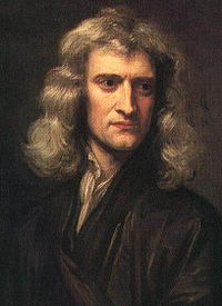
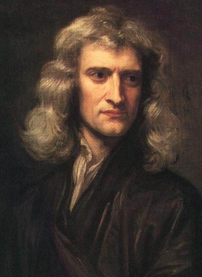
The product rule and chain rule, the notion of higher derivatives, Taylor series, and analytical functions were introduced by Isaac Newton in an idiosyncratic notation which he used to solve problems of mathematical physics. In his publications, Newton rephrased his ideas to suit the mathematical idiom of the time, replacing calculations with infinitesimals by equivalent geometrical arguments which were considered beyond reproach. He used the methods of calculus to solve the problem of planetary motion, the shape of the surface of a rotating fluid, the oblateness of the earth, the motion of a weight sliding on a cycloid, and many other problems discussed in his Principia Mathematica (1687). In other work, he developed series expansions for functions, including fractional and irrational powers, and it was clear that he understood the principles of the Taylor series. He did not publish all these discoveries, and at this time infinitesimal methods were still considered disreputable.

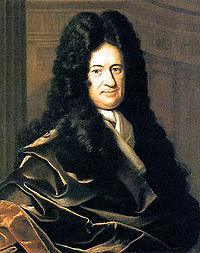Gottfried Wilhelm Leibniz was the first to publish his results on the development of calculus.

These ideas were systematized into a true calculus of infinitesimals by Gottfried Wilhelm Leibniz, who was originally accused of plagiarism by Newton.^[9] He is now regarded as an independent inventor of and contributor to calculus. His contribution was to provide a clear set of rules for manipulating infinitesimal quantities, allowing the computation of second and higher derivatives, and providing the product rule and chain rule, in their differential and integral forms. Unlike Newton, Leibniz paid a lot of attention to the formalism, often spending days determining appropriate symbols for concepts.

Leibniz and Newton are usually both credited with the invention of calculus. Newton was the first to apply calculus to general physics and Leibniz developed much of the notation used in calculus today. The basic insights that both Newton and Leibniz provided were the laws of differentiation and integration, second and higher derivatives, and the notion of an approximating polynomial series. By Newton's time, the fundamental theorem of calculus was known.

When Newton and Leibniz first published their results, there was great controversy over which mathematician (and therefore which country) deserved credit. Newton derived his results first, but Leibniz published first. Newton claimed Leibniz stole ideas from his unpublished notes, which Newton had shared with a few members of the Royal Society. This controversy divided English-speaking mathematicians from continental mathematicians for many years, to the detriment of English mathematics. A careful examination of the papers of Leibniz and Newton shows that they arrived at their results independently, with Leibniz starting first with integration and Newton with differentiation. Today, both Newton and Leibniz are given credit for developing calculus independently. It is Leibniz, however, who gave the new discipline its name. Newton called his calculus "the science of fluxions".

Since the time of Leibniz and Newton, many mathematicians have contributed to the continuing development of calculus. One of the first and most complete works on finite and infinitesimal analysis was written in 1748 by Maria Gaetana Agnesi.^[10]

Maria Gaetana Agnesi

Foundations

In mathematics, foundations refers to the rigorous development of a subject from precise axioms and definitions. In early calculus the use of infinitesimal quantities was thought unrigorous, and was fiercely criticized by a number of authors, most notably Michel Rolle and Bishop Berkeley. Berkeley famously described infinitesimals as the ghosts of departed quantities in his book The Analyst in 1734. Working out a rigorous foundation for calculus occupied mathematicians for much of the century following Newton and Leibniz and is still to some extent an active area of research today.

Several mathematicians, including Maclaurin, attempted to prove the soundness of using infinitesimals, but it would be 150 years later, due to the work of Cauchy and Weierstrass, where a means was finally found to avoid mere "notions" of infinitely small quantities and the foundations of differential and integral calculus were made firm. In Cauchy's writing, we find a versatile spectrum of foundational approaches, including a definition of continuity in terms of infinitesimals, and a (somewhat imprecise) prototype of an (ε, δ)-definition of limit in the definition of differentiation. In his work Weierstrass formalized the concept of limit and eliminated infinitesimals. Following the work of Weierstrass, it eventually became common to base calculus on limits instead of infinitesimal quantities. Bernhard Riemann used these ideas to give a precise definition of the integral. It was also during this period that the ideas of calculus were generalized to Euclidean space and the complex plane.

In modern mathematics, the foundations of calculus are included in the field of real analysis, which contains full definitions and proofs of the theorems of calculus. The reach of calculus has also been greatly extended. Henri Lebesgue invented measure theory and used it to define integrals of all but the most pathological functions. Laurent Schwartz introduced Distributions, which can be used to take the derivative of any function whatsoever.

Limits are not the only rigorous approach to the foundation of calculus. An alternative is Abraham Robinson's nonstandard analysis. Robinson's approach, developed in the 1960s, uses technical machinery from mathematical logic to augment the real number system with infinitesimal and infinite numbers, as in the original Newton-Leibniz conception. The resulting numbers are called hyperreal numbers, and they can be used to give a Leibniz-like development of the usual rules of calculus.

Significance

While some of the ideas of calculus were developed earlier in Egypt, Greece, China, India, Iraq, Persia, and Japan, the modern use of calculus began in Europe, during the 17th century, when Isaac Newton and Gottfried Wilhelm Leibniz built on the work of earlier mathematicians to introduce its basic principles. The development of calculus was built on earlier concepts of instantaneous motion and area underneath curves.

Applications of differential calculus include computations involving velocity and acceleration, the slope of a curve, and optimization. Applications of integral calculus include computations involving area, volume, arc length, center of mass, work, and pressure. More advanced applications include power series and Fourier series.

Calculus is also used to gain a more precise understanding of the nature of space, time, and motion. For centuries, mathematicians and philosophers wrestled with paradoxes involving division by zero or sums of infinitely many numbers. These questions arise in the study of motion and area. The ancient Greek philosopher Zeno of Elea gave several famous examples of such paradoxes. Calculus provides tools, especially the limit and the infinite series, which resolve the paradoxes.

Principles

Limits and infinitesimals

Main articles: Limit of a function, Infinitesimal, and Infinitesimal Calculus

Calculus is usually developed by manipulating very small quantities. Historically, the first method of doing so was by infinitesimals. These are objects which can be treated like numbers but which are, in some sense, "infinitely small". An infinitesimal number dx could be greater than 0, but less than any number in the sequence 1, 1/2, 1/3, ... and less than any positive real number. Any integer multiple of an infinitesimal is still infinitely small, i.e., infinitesimals do not satisfy the Archimedean property. From this point of view, calculus is a collection of techniques for manipulating infinitesimals. This approach fell out of favor in the 19th century because it was difficult to make the notion of an infinitesimal precise. However, the concept was revived in the 20th century with the introduction of non-standard analysis and smooth infinitesimal analysis, which provided solid foundations for the manipulation of infinitesimals.

In the 19th century, infinitesimals were replaced by limits. Limits describe the value of a function at a certain input in terms of its values at nearby input. They capture small-scale behavior, just like infinitesimals, but use the ordinary real number system. In this treatment, calculus is a collection of techniques for manipulating certain limits. Infinitesimals get replaced by very small numbers, and the infinitely small behavior of the function is found by taking the limiting behavior for smaller and smaller numbers. Limits are the easiest way to provide rigorous foundations for calculus, and for this reason they are the standard approach.

Differential calculus

Main article: Differential calculus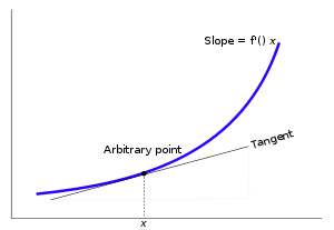

Tangent line at (x, f(x)). The derivative f′(x) of a curve at a point is the slope (rise over run) of the line tangent to that curve at that point.

Differential calculus is the study of the definition, properties, and applications of the derivative of a function. The process of finding the derivative is called differentiation. Given a function and a point in the domain, the derivative at that point is a way of encoding the small-scale behavior of the function near that point. By finding the derivative of a function at every point in its domain, it is possible to produce a new function, called the derivative function or just the derivative of the original function. In mathematical jargon, the derivative is a linear operator which inputs a function and outputs a second function. This is more abstract than many of the processes studied in elementary algebra, where functions usually input a number and output another number. For example, if the doubling function is given the input three, then it outputs six, and if the squaring function is given the input three, then it outputs nine. The derivative, however, can take the squaring function as an input. This means that the derivative takes all the information of the squaring function—such as that two is sent to four, three is sent to nine, four is sent to sixteen, and so on—and uses this information to produce another function. (The function it produces turns out to be the doubling function.)

The most common symbol for a derivative is an apostrophe-like mark called prime. Thus, the derivative of the function of f is f′, pronounced "f prime." For instance, if f(x) = x² is the squaring function, then f′(x) = 2x is its derivative, the doubling function.

If the input of the function represents time, then the derivative represents change with respect to time. For example, if f is a function that takes a time as input and gives the position of a ball at that time as output, then the derivative of f is how the position is changing in time, that is, it is the velocity of the ball.

If a function is linear (that is, if the graph of the function is a straight line), then the function can be written as y = mx + b, where x is the independent variable, y is the dependent variable, b is the y-intercept, and:

$m= \frac{\text{rise}}{\text{run}}= \frac{\text{change in } y}{\text{change in } x} = \frac{\Delta y}{\Delta x}.$

This gives an exact value for the slope of a straight line. If the graph of the function is not a straight line, however, then the change in y divided by the change in x varies. Derivatives give an exact meaning to the notion of change in output with respect to change in input. To be concrete, let f be a function, and fix a point a in the domain of f. (a, f(a)) is a point on the graph of the function. If h is a number close to zero, then a + h is a number close to a. Therefore (a + h, f(a + h)) is close to (a, f(a)). The slope between these two points is

$m = \frac{f(a+h) - f(a)}{(a+h) - a} = \frac{f(a+h) - f(a)}{h}.$

This expression is called a difference quotient. A line through two points on a curve is called a secant line, so m is the slope of the secant line between (a, f(a)) and (a + h, f(a + h)). The secant line is only an approximation to the behavior of the function at the point a because it does not account for what happens between a and a + h. It is not possible to discover the behavior at a by setting h to zero because this would require dividing by zero, which is impossible. The derivative is defined by taking the limit as h tends to zero, meaning that it considers the behavior of f for all small values of h and extracts a consistent value for the case when h equals zero:

$\lim_{h \to 0}{f(a+h) - f(a)\over{h}}.$

Geometrically, the derivative is the slope of the tangent line to the graph of f at a. The tangent line is a limit of secant lines just as the derivative is a limit of difference quotients. For this reason, the derivative is sometimes called the slope of the function f.

Here is a particular example, the derivative of the squaring function at the input 3. Let f(x) = x² be the squaring function.

The derivative f′(x) of a curve at a point is the slope of the line tangent to that curve at that point. This slope is determined by considering the limiting value of the slopes of secant lines. Here the function involved (drawn in red) is f(x) = x³ − x. The tangent line (in green) which passes through the point (−3/2, −15/8) has a slope of 23/4. Note that the vertical and horizontal scales in this image are different.

$\begin{align}f'(3) &=\lim_{h \to 0}{(3+h)^2 - 3^2\over{h}} \\ &=\lim_{h \to 0}{9 + 6h + h^2 - 9\over{h}} \\ &=\lim_{h \to 0}{6h + h^2\over{h}} \\ &=\lim_{h \to 0} (6 + h) \\ &= 6. \end{align}$

The slope of tangent line to the squaring function at the point (3,9) is 6, that is to say, it is going up six times as fast as it is going to the right. The limit process just described can be performed for any point in the domain of the squaring function. This defines the derivative function of the squaring function, or just the derivative of the squaring function for short. A similar computation to the one above shows that the derivative of the squaring function is the doubling function.

Leibniz notation

Main article: Leibniz's notation

A common notation, introduced by Leibniz, for the derivative in the example above is

$\begin{align} y&=x^2 \\ \frac{dy}{dx}&=2x. \end{align}$

In an approach based on limits, the symbol dy/dx is to be interpreted not as the quotient of two numbers but as a shorthand for the limit computed above. Leibniz, however, did intend it to represent the quotient of two infinitesimally small numbers, dy being the infinitesimally small change in y caused by an infinitesimally small change dx applied to x. We can also think of d/dx as a differentiation operator, which takes a function as an input and gives another function, the derivative, as the output. For example:

$\frac{d}{dx}(x^2)=2x.$

In this usage, the dx in the denominator is read as "with respect to x". Even when calculus is developed using limits rather than infinitesimals, it is common to manipulate symbols like dx and dy as if they were real numbers; although it is possible to avoid such manipulations, they are sometimes notationally convenient in expressing operations such as the total derivative.

Integral calculus

Main article: Integral

Integral calculus is the study of the definitions, properties, and applications of two related concepts, the indefinite integral and the definite integral. The process of finding the value of an integral is called integration. In technical language, integral calculus studies two related linear operators.

The indefinite integral is the antiderivative, the inverse operation to the derivative. F is an indefinite integral of f when f is a derivative of F. (This use of upper- and lower-case letters for a function and its indefinite integral is common in calculus.)

The definite integral inputs a function and outputs a number, which gives the area between the graph of the input and the x-axis. The technical definition of the definite integral is the limit of a sum of areas of rectangles, called a Riemann sum.

A motivating example is the distances traveled in a given time.

$\mathrm{Distance} = \mathrm{Speed} \cdot \mathrm{Time}$

If the speed is constant, only multiplication is needed, but if the speed changes, then we need a more powerful method of finding the distance. One such method is to approximate the distance traveled by breaking up the time into many short intervals of time, then multiplying the time elapsed in each interval by one of the speeds in that interval, and then taking the sum (a Riemann sum) of the approximate distance traveled in each interval. The basic idea is that if only a short time elapses, then the speed will stay more or less the same. However, a Riemann sum only gives an approximation of the distance traveled. We must take the limit of all such Riemann sums to find the exact distance traveled.

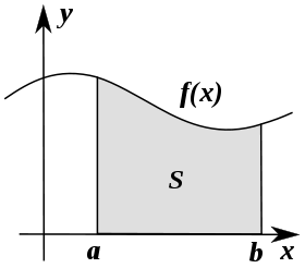Integration can be thought of as measuring the area under a curve, defined by f(x), between two points (here a and b).

If f(x) in the diagram on the left represents speed as it varies over time, the distance traveled (between the times represented by a and b) is the area of the shaded region s.

To approximate that area, an intuitive method would be to divide up the distance between a and b into a number of equal segments, the length of each segment represented by the symbol Δx. For each small segment, we can choose one value of the function f(x). Call that value h. Then the area of the rectangle with base Δx and height h gives the distance (time Δx multiplied by speed h) traveled in that segment. Associated with each segment is the average value of the function above it, f(x)=h. The sum of all such rectangles gives an approximation of the area between the axis and the curve, which is an approximation of the total distance traveled. A smaller value for Δx will give more rectangles and in most cases a better approximation, but for an exact answer we need to take a limit as Δx approaches zero.

The symbol of integration is $\int \,$, an elongated S (the S stands for "sum"). The definite integral is written as:

$\int_a^b f(x)\, dx.$

and is read "the integral from a to b of f-of-x with respect to x." The Leibniz notation dx is intended to suggest dividing the area under the curve into an infinite number of rectangles, so that their width Δx becomes the infinitesimally small dx. In a formulation of the calculus based on limits, the notation

$\int_a^b \ldots\, dx$

is to be understood as an operator that takes a function as an input and gives a number, the area, as an output; dx is not a number, and is not being multiplied by f(x).

The indefinite integral, or antiderivative, is written:

$\int f(x)\, dx.$

Functions differing by only a constant have the same derivative, and therefore the antiderivative of a given function is actually a family of functions differing only by a constant. Since the derivative of the function y = x² + C, where C is any constant, is y′ = 2x, the antiderivative of the latter is given by:

$\int 2x\, dx = x^2 + C.$

An undetermined constant like C in the antiderivative is known as a constant of integration.

Fundamental theorem

Main article: Fundamental theorem of calculus

The fundamental theorem of calculus states that differentiation and integration are inverse operations. More precisely, it relates the values of antiderivatives to definite integrals. Because it is usually easier to compute an antiderivative than to apply the definition of a definite integral, the Fundamental Theorem of Calculus provides a practical way of computing definite integrals. It can also be interpreted as a precise statement of the fact that differentiation is the inverse of integration.

The Fundamental Theorem of Calculus states: If a function f is continuous on the interval [a, b] and if F is a function whose derivative is f on the interval (a, b), then

$\int_{a}^{b} f(x)\,dx = F(b) - F(a).$

Furthermore, for every x in the interval (a, b),

$\frac{d}{dx}\int_a^x f(t)\, dt = f(x).$

This realization, made by both Newton and Leibniz, who based their results on earlier work by Isaac Barrow, was key to the massive proliferation of analytic results after their work became known. The fundamental theorem provides an algebraic method of computing many definite integrals—without performing limit processes—by finding formulas for antiderivatives. It is also a prototype solution of a differential equation. Differential equations relate an unknown function to its derivatives, and are ubiquitous in the sciences.

Applications

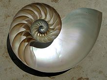The logarithmic spiral of the Nautilus shell is a classical image used to depict the growth and change related to calculus

Calculus is used in every branch of the physical sciences, actuarial science, computer science, statistics, engineering, economics, business, medicine, demography, and in other fields wherever a problem can be mathematically modeled and an optimal solution is desired. It allows one to go from (non-constant) rates of change to the total change or vice versa, and many times in studying a problem we know one and are trying to find the other.

Physics makes particular use of calculus; all concepts in classical mechanics and electromagnetism are interrelated through calculus. The mass of an object of known density, the moment of inertia of objects, as well as the total energy of an object within a conservative field can be found by the use of calculus. An example of the use of calculus in mechanics is Newton's second law of motion: historically stated it expressly uses the term "rate of change" which refers to the derivative saying The rate of change of momentum of a body is equal to the resultant force acting on the body and is in the same direction. Commonly expressed today as Force = Mass × acceleration, it involves differential calculus because acceleration is the time derivative of velocity or second time derivative of trajectory or spatial position. Starting from knowing how an object is accelerating, we use calculus to derive its path.

Maxwell's theory of electromagnetism and Einstein's theory of general relativity are also expressed in the language of differential calculus. Chemistry also uses calculus in determining reaction rates and radioactive decay. In biology, population dynamics starts with reproduction and death rates to model population changes.

Calculus can be used in conjunction with other mathematical disciplines. For example, it can be used with linear algebra to find the "best fit" linear approximation for a set of points in a domain. Or it can be used in probability theory to determine the probability of a continuous random variable from an assumed density function. In analytic geometry, the study of graphs of functions, calculus is used to find high points and low points (maxima and minima), slope, concavity and inflection points.

Green's Theorem, which gives the relationship between a line integral around a simple closed curve C and a double integral over the plane region D bounded by C, is applied in an instrument known as a planimeter which is used to calculate the area of a flat surface on a drawing. For example, it can be used to calculate the amount of area taken up by an irregularly shaped flower bed or swimming pool when designing the layout of a piece of property.

Discrete Green's Theorem, which gives the relationship between a double integral of a function around a simple closed rectangular curve C and a linear combination of the antiderivative's values at corner points along the edge of the curve, allows fast calculation of sums of values in rectangular domains. For example, it can be used to efficiently calculate sums of rectangular domains in images, in order to rapidly extract features and detect object - see also the summed area table algorithm.

In the realm of medicine, calculus can be used to find the optimal branching angle of a blood vessel so as to maximize flow. From the decay laws for a particular drug's elimination from the body, it's used to derive dosing laws. In nuclear medicine, it's used to build models of radiation transport in targeted tumor therapies.

In economics, calculus allows for the determination of maximal profit by providing a way to easily calculate both marginal cost and marginal revenue.

Calculus is also used to find approximate solutions to equations; in practice it's the standard way to solve differential equations and do root finding in most applications. Examples are methods such as Newton's method, fixed point iteration, and linear approximation. For instance, spacecraft use a variation of the Euler method to approximate curved courses within zero gravity environments.

See also

	Mathematics portal
	Analysis portal

Main article: Outline of calculus

Lists

• List of calculus topics
• List of derivatives and integrals in alternative calculi
• List of differentiation identities
• Publications in calculus
• Table of integrals

Related topics

• Calculus of finite differences
• Calculus with polynomials
• Complex analysis
• Differential equation
• Differential geometry
• Elementary Calculus: An Infinitesimal Approach
• Fourier series
• Integral equation
• Mathematical analysis
• Multivariable calculus
• Non-classical analysis
• Non-standard analysis
• Non-standard calculus
• Precalculus (mathematical education)
• Product integral
• Stochastic calculus
• Taylor series

References

Notes

1. ^ Latorre, Donald R.; Kenelly, John W.; Reed, Iris B.; Biggers, Sherry (2007), Calculus Concepts: An Applied Approach to the Mathematics of Change, Cengage Learning, p. 2, ISBN 0-618-78981-2, http://books.google.com/books?id=bQhX-3k0LS8C , Chapter 1, p 2
2. ^ Morris Kline, Mathematical thought from ancient to modern times, Vol. I
3. ^ Archimedes, Method, in The Works of Archimedes ISBN 978-0-521-66160-7
4. ^ Dun, Liu; Fan, Dainian; Cohen, Robert Sonné (1966). A comparison of Archimdes' and Liu Hui's studies of circles. Chinese studies in the history and philosophy of science and technology. 130. Springer. p. 279. ISBN 0-792-33463-9. http://books.google.com/books?id=jaQH6_8Ju-MC. , Chapter , p. 279
5. ^ Zill, Dennis G.; Wright, Scott; Wright, Warren S. (2009). Calculus: Early Transcendentals (3 ed.). Jones & Bartlett Learning. p. xxvii. ISBN 0-763-75995-3. http://books.google.com/books?id=R3Hk4Uhb1Z0C. , Extract of page 27
6. ^ http://www-history.mcs.st-andrews.ac.uk/HistTopics/Indian_mathematics.html
7. ^ von Neumann, J., "The Mathematician", in Heywood, R. B., ed., The Works of the Mind, University of Chicago Press, 1947, pp. 180–196. Reprinted in Bródy, F., Vámos, T., eds., The Neumann Compedium, World Scientific Publishing Co. Pte. Ltd., 1995, ISBN 9810222017, pp. 618–626.
8. ^ André Weil: Number theory. An approach through history. From Hammurapi to Legendre. Birkhauser Boston, Inc., Boston, MA, 1984, ISBN 0817645659, p. 28.
9. ^ Leibniz, Gottfried Wilhelm. The Early Mathematical Manuscripts of Leibniz. Cosimo, Inc., 2008. Page 228. Copy
10. ^ Unlu, Elif (April 1995). "Maria Gaetana Agnesi". Agnes Scott College. http://www.agnesscott.edu/lriddle/women/agnesi.htm. 

Books

• Larson, Ron, Bruce H. Edwards (2010). "Calculus", 9th ed., Brooks Cole Cengage Learning. ISBN 9780547167022
• McQuarrie, Donald A. (2003). Mathematical Methods for Scientists and Engineers, University Science Books. ISBN 9781891389245
• Stewart, James (2008). Calculus: Early Transcendentals, 6th ed., Brooks Cole Cengage Learning. ISBN 9780495011668
• Thomas, George B., Maurice D. Weir, Joel Hass, Frank R. Giordano (2008), "Calculus", 11th ed., Addison-Wesley. ISBN 0-321-48987-X

Other resources

Further reading

• Boyer, Carl Benjamin (1949). The History of the Calculus and its Conceptual Development. Hafner. Dover edition 1959, ISBN 0-486-60509-4
• Courant, Richard ISBN 978-3540650584 Introduction to calculus and analysis 1.
• Edmund Landau. ISBN 0-8218-2830-4 Differential and Integral Calculus, American Mathematical Society.
• Robert A. Adams. (1999). ISBN 978-0-201-39607-2 Calculus: A complete course.
• Albers, Donald J.; Richard D. Anderson and Don O. Loftsgaarden, ed. (1986) Undergraduate Programs in the Mathematics and Computer Sciences: The 1985-1986 Survey, Mathematical Association of America No. 7.
• John Lane Bell: A Primer of Infinitesimal Analysis, Cambridge University Press, 1998. ISBN 978-0-521-62401-5. Uses synthetic differential geometry and nilpotent infinitesimals.
• Florian Cajori, "The History of Notations of the Calculus." Annals of Mathematics, 2nd Ser., Vol. 25, No. 1 (Sep., 1923), pp. 1–46.
• Leonid P. Lebedev and Michael J. Cloud: "Approximating Perfection: a Mathematician's Journey into the World of Mechanics, Ch. 1: The Tools of Calculus", Princeton Univ. Press, 2004.
• Cliff Pickover. (2003). ISBN 978-0-471-26987-8 Calculus and Pizza: A Math Cookbook for the Hungry Mind.
• Michael Spivak. (September 1994). ISBN 978-0-914098-89-8 Calculus. Publish or Perish publishing.
• Tom M. Apostol. (1967). ISBN 9780471000051 Calculus, Volume 1, One-Variable Calculus with an Introduction to Linear Algebra. Wiley.
• Tom M. Apostol. (1969). ISBN 9780471000075 Calculus, Volume 2, Multi-Variable Calculus and Linear Algebra with Applications. Wiley.
• Silvanus P. Thompson and Martin Gardner. (1998). ISBN 978-0-312-18548-0 Calculus Made Easy.
• Mathematical Association of America. (1988). Calculus for a New Century; A Pump, Not a Filter, The Association, Stony Brook, NY. ED 300 252.
• Thomas/Finney. (1996). ISBN 978-0-201-53174-9 Calculus and Analytic geometry 9th, Addison Wesley.
• Weisstein, Eric W. "Second Fundamental Theorem of Calculus." From MathWorld—A Wolfram Web Resource.
• Howard Anton,Irl Bivens,Stephen Davis:"Calculus",John Willey and Sons Pte. Ltd.,2002.ISBN 978-81-265-1259-1

Online books

• Crowell, B. (2003). "Calculus" Light and Matter, Fullerton. Retrieved 6 May 2007 from http://www.lightandmatter.com/calc/calc.pdf
• Garrett, P. (2006). "Notes on first year calculus" University of Minnesota. Retrieved 6 May 2007 from http://www.math.umn.edu/~garrett/calculus/first_year/notes.pdf
• Faraz, H. (2006). "Understanding Calculus" Retrieved 6 May 2007 from Understanding Calculus, URL http://www.understandingcalculus.com/ (HTML only)
• Keisler, H. J. (2000). "Elementary Calculus: An Approach Using Infinitesimals" Retrieved 29 August 2010 from http://www.math.wisc.edu/~keisler/calc.html
• Mauch, S. (2004). "Sean's Applied Math Book" California Institute of Technology. Retrieved 6 May 2007 from http://www.cacr.caltech.edu/~sean/applied_math.pdf
• Sloughter, Dan (2000). "Difference Equations to Differential Equations: An introduction to calculus". Retrieved 17 March 2009 from http://synechism.org/drupal/de2de/
• Stroyan, K.D. (2004). "A brief introduction to infinitesimal calculus" University of Iowa. Retrieved 6 May 2007 from http://www.math.uiowa.edu/~stroyan/InfsmlCalculus/InfsmlCalc.htm (HTML only)
• Strang, G. (1991). "Calculus" Massachusetts Institute of Technology. Retrieved 6 May 2007 from http://ocw.mit.edu/ans7870/resources/Strang/strangtext.htm
• Smith, William V. (2001). "The Calculus" Retrieved 4 July 2008 [1] (HTML only).

External links

• Weisstein, Eric W., "Calculus" from MathWorld.
• Topics on Calculus at PlanetMath.
• Calculus Made Easy (1914) by Silvanus P. Thompson Full text in PDF
• Calculus on In Our Time at the BBC. (listen now)
• Calculus.org: The Calculus page at University of California, Davis – contains resources and links to other sites
• COW: Calculus on the Web at Temple University – contains resources ranging from pre-calculus and associated algebra
• Earliest Known Uses of Some of the Words of Mathematics: Calculus & Analysis
• Online Integrator (WebMathematica) from Wolfram Research
• The Role of Calculus in College Mathematics from ERICDigests.org
• OpenCourseWare Calculus from the Massachusetts Institute of Technology
• Infinitesimal Calculus – an article on its historical development, in Encyclopaedia of Mathematics, Michiel Hazewinkel ed. .
• Elements of Calculus I and Calculus II for Business, OpenCourseWare from the University of Notre Dame with activities, exams and interactive applets.
• Calculus for Beginners and Artists by Daniel Kleitman, MIT
• Calculus Problems and Solutions by D. A. Kouba
• Solved problems in calculus
• Video explanations and solved problems in calculus Raymond, CUNY