Power dividers and directional couplers

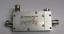A 10 dB 1.7–2.2 GHz directional coupler. From left to right: input, coupled, isolated (terminated with a load), and transmitted port.

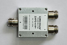A 3 dB 2.0–4.2 GHz power divider/combiner.

Power dividers (also power splitters and, when used in reverse, power combiners) and directional couplers are passive devices used in the field of radio technology. They couple a defined amount of the electromagnetic power in a transmission line to another port where it can be used in another circuit. An essential feature of directional couplers is that they only couple power flowing in one direction. Power entering the output port is not coupled.

Directional couplers are most frequently constructed from two coupled transmission lines set close enough together such that energy passing through one is coupled to the other. This technique is favoured due to the microwave frequencies the devices are commonly employed with. However, lumped component devices are also possible at lower frequencies. Also at microwave frequencies, particularly the higher bands, waveguide designs can be used. Many of these waveguide couplers correspond to one of the conducting transmission line designs, but there are also types that are unique to waveguide.

Directional couplers and power dividers have many applications, these include; providing a signal sample for measurement or monitoring, feedback, combining feeds to and from antennae, antenna beam forming, providing taps for cable distributed systems such as cable TV, and separating transmitted and received signals on telephone lines.

Notation and symbols

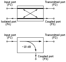Figure 1. Two symbols used for directional couplers

The symbols most often used for directional couplers are shown in figure 1. The symbol may have marked on it a number in dB: this refers to the coupling factor of the coupler. Directional couplers have four ports. Port 1 is the input port where power is applied. Port 3 is the coupled port where a portion of the power applied to port 1 appears. Port 2 is the transmitted port where the power from port 1 is outputted, less the portion that went to port 3. Directional couplers are frequently symmetrical so there also exists port 4, the isolated port. A portion of the power applied to port 2 will be coupled to port 4. However, the device is not normally used in this mode and port 4 is usually terminated with a matched load (typically 50 ohms). This termination can be internal to the device and port 4 is not accessible to the user. Effectively, this results in a 3-port device, hence the utility of the second symbol for directional couplers in figure 1.^[1]

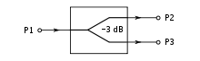Figure 2. Symbol for power divider

Symbols of the form;

$P_\mathrm {a,b} \$

in this article have the meaning "parameter P at port a due to an input at port b".

A symbol for power dividers is shown in figure 2. Power dividers and directional couplers are in all essentials the same class of device. Directional coupler tends to be used for 4-port devices that are only loosely coupled – that is, only a small fraction of the input power appears at the coupled port. Power divider is used for devices with tight coupling (commonly, a power divider will provide half the input power at each of its output ports – a 3 dB divider) and is usually considered a 3-port device.^[2]

Parameters

Common properties desired for all directional couplers are wide operational bandwidth, high directivity, and a good impedance match at all ports when the other ports are terminated in matched loads. Some of these, and other, general characteristics are discussed below.^[3]

Coupling factor

The coupling factor is defined as: $C_{3,1} = -10 \log{\left( \frac{P_3}{P_1} \right)} \quad \rm{dB}$

where P₁ is the input power at port 1 and P₃ is the output power from the coupled port (see figure 1).

The coupling factor represents the primary property of a directional coupler. Coupling factor is a negative quantity, it cannot exceed 0 dB for a passive device, and in practice does not exceed −3 dB since more than this would result in more power output from the coupled port than power from the transmitted port – in effect their roles would be reversed. Although a negative quantity, the minus sign is frequently dropped (but still implied) in running text and diagrams and a few authors^[4] go so far as to define it as a positive quantity. Coupling is not constant, but varies with frequency. While different designs may reduce the variance, a perfectly flat coupler theoretically cannot be built. Directional couplers are specified in terms of the coupling accuracy at the frequency band center.^[5]

Loss

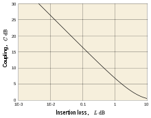Figure 3. Graph of insertion loss due to coupling

In an ideal directional coupler, the main line loss from port 1 to port 2 (P₁ – P₂) due to power coupled to the coupled output port is:

Insertion loss: $L_{2,1} = - 10 \log{\left(1 - \frac{P_3}{P_1} \right)} \quad \rm{dB}$

The actual directional coupler loss will be a combination of coupling loss, dielectric loss, conductor loss, and VSWR loss. Depending on the frequency range, coupling loss becomes less significant above 15 dB coupling where the other losses constitute the majority of the total loss. The theoretical insertion loss (dB) vs coupling (dB) for a dissipationless coupler is shown in the graph of figure 3 and the table below.^[6]

Insertion loss due to coupling

Coupling	Insertion loss
dB	dB
3	3.00
6	1.25
10	0.458
20	0.0436
30	0.00435

Isolation

Isolation of a directional coupler can be defined as the difference in signal levels in dB between the input port and the isolated port when the two other ports are terminated by matched loads, or:

Isolation: $I_{4,1} = -10 \log{\left( \frac{P_4}{P_1} \right)} \quad \rm{dB}$

Isolation can also be defined between the two output ports. In this case, one of the output ports is used as the input; the other is considered the output port while the other two ports (input and isolated) are terminated by matched loads.

Consequently: $I_{3,2} = -10 \log{\left( \frac{P_3}{P_2} \right)} \quad \rm{dB}$

The isolation between the input and the isolated ports may be different from the isolation between the two output ports. For example, the isolation between ports 1 and 4 can be 30 dB while the isolation between ports 2 and 3 can be a different value such as 25 dB. Isolation can be estimated from the coupling plus return loss. The isolation should be as high as possible. In actual couplers the isolated port is never completely isolated. Some RF power will always be present. Waveguide directional couplers will have the best isolation.^[7]

Directivity

Directivity is directly related to isolation. It is defined as:

Directivity: $D_{3,4} = -10 \log{\left( \frac{P_4}{P_3} \right)} = -10 \log{\left( \frac{P_4}{P_1} \right)}+ 10 \log{\left( \frac{P_3}{P_1} \right)}\quad \rm{dB}$

where: P₃ is the output power from the coupled port and P₄ is the power output from the isolated port.

The directivity should be as high as possible. The directivity is very high at the design frequency and is a more sensitive function of frequency because it depends on the cancellation of two wave components. Waveguide directional couplers will have the best directivity. Directivity is not directly measurable, and is calculated from the difference of the isolation and coupling measurements as:^[8]

$D_{3,4} = I_{4,1} - C_{3,1} \quad \rm{dB}$

S-parameters

The S-matrix for an ideal (infinite isolation and perfectly matched) symmetrical directional coupler is given by,

$\mathbf S = \begin{bmatrix} 0 & \tau & \kappa & 0 \\ \tau & 0 & 0 & \kappa \\ \kappa & 0 & 0 & \tau \\ 0 & \kappa & \tau & 0 \end{bmatrix}$

$\tau \$ is the transmission coefficient and,

$\kappa \$ is the coupling coefficient

In general, $\tau \$ and $\kappa \$ are complex, frequency dependent, numbers. The zeroes on the matrix main diagonal are a consequence of perfect matching – power input to any port is not reflected back to that same port. The zeroes on the matrix antidiagonal are a consequence of perfect isolation between the input and isolated port.

For a passive lossless directional coupler, we must in addition have,

$\tau \overline{\tau} + \kappa \overline{\kappa} = 1$

since the power entering the input port must all leave by one of the other two ports.^[9]

Insertion loss is related to $\tau \$ by;

$L (\mathrm {dB}) = -20 \log | \tau | \$

Coupling factor is related to $\kappa \$ by;

$C (\mathrm {dB}) = 20 \log | \kappa | \$

Non-zero main diagonal entries are related to return loss, and non-zero antidiagonal entries are related to isolation by similar expressions.

Some authors define the port numbers with ports 3 and 4 interchanged. This results in a scattering matrix that is no longer all-zeroes on the antidiagonal.^[10]

Amplitude balance

This terminology defines the power difference in dB between the two output ports of a 3 dB hybrid. In an ideal hybrid circuit, the difference should be 0 dB. However, in a practical device the amplitude balance is frequency dependent and departs from the ideal 0 dB difference.^[11]

Phase balance

The phase difference between the two output ports of a hybrid coupler should be 0°, 90°, or 180° depending on the type used. However, like amplitude balance, the phase difference is sensitive to the input frequency and typically will vary a few degrees.^[12]

Transmission line types

Directional couplers

Coupled transmission lines

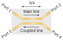Figure 4. Single section λ/4 directional coupler

The most common form of directional coupler is a pair of coupled transmission lines. They can be realised in a number of technologies including coaxial and the planar technologies (stripline and microstrip). An implementation in stripline is shown in figure 4 of a quarter-wavelength (λ/4) directional coupler. The power on the coupled line flows in the opposite direction to the power on the main line, hence the port arrangement is not the same as shown in figure 1, but the numbering remains the same. For this reason it is sometimes called a backward coupler.^[13]

The term main line refers to the section between ports 1 and 2 and coupled line to the section between ports 3 and 4. Since the directional coupler is a linear device, the notations on figure 1 are arbitrary. Any port can be the input, (an example is seen in figure 20) which will result in the directly connected port being the transmitted port, the adjacent port being the coupled port, and the diagonal port being the isolated port. On some directional couplers, the main line is designed for high power operation (large connectors), while the coupled port may use a small SMA connector. The internal load power rating may also limit operation on the coupled line.^[14]

Figure 5. Short section directional coupler

Figure 6. Short section directional coupler with 50 Ω main line and 100 Ω coupled line

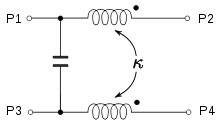Figure 7. Lumped element equivalent circuit of the couplers depicted in figures 5 and 6

Accuracy of coupling factor depends on the dimensional tolerances for the spacing of the two coupled lines. For planar printed technologies this comes down to the resolution of the printing process which determines the minimum track width that can be produced and also puts a limit on how close the lines can be placed to each other. This becomes a problem when very tight coupling is required and 3 dB couplers often use a different design. However, tightly coupled lines can be produced in air stripline which also permits manufacture by printed planar technology. In this design the two lines are printed on opposite sides of the dielectric rather than side by side. The coupling of the two lines across their width is much greater than the coupling when they are edge-on to each other.^[15]

The λ/4 coupled line design is good for coaxial and stripline implementations but does not work so well in the now popular microstrip format, although designs do exist. The reason for this is that microstrip is not a homogenous medium – there are two different mediums above and below the transmission strip. This leads to transmission modes other than the usual TEM mode found in conductive circuits. The propagation velocities of even and odd modes are different leading to signal dispersion. A better solution for microstrip is a coupled line much shorter than λ/4, shown in figure 5, but this has the disadvantage of a coupling factor which rises noticeably with frequency. A variation of this design sometimes encountered has the coupled line a higher impedance than the main line such as shown in figure 6. This design is advantageous where the coupler is being fed to a detector for power monitoring. The higher impedance line results in a higher RF voltage for a given main line power making the work of the detector diode easier.^[16]

The frequency range specified by manufacturers is that of the coupled line. The main line response is much wider: for instance a coupler specified as 2–4 GHz might have a main line which could operate at 1–5 GHz. As with all distributed element circuits, the coupled response is periodic with frequency. For example, a λ/4 coupled line coupler will have responses at nλ/4 where n is an odd integer.^[17]

A single λ/4 coupled section is good for bandwidths of less than an octave. To achieve greater bandwidths multiple λ/4 coupling sections are used. The design of such couplers proceeds in much the same way as the design of distributed element filters. The sections of the coupler are treated as being sections of a filter, and by adjusting the coupling factor of each section the coupled port can be made to have any of the classic filter responses such as maximally flat (Butterworth filter), equal-ripple (Cauer filter), or a specified-ripple Chebychev filter response. Ripple in this context refers to the maximum variation in output of the coupled port in its passband, usually quoted as plus or minus a value in dB from the nominal coupling factor.^[18]

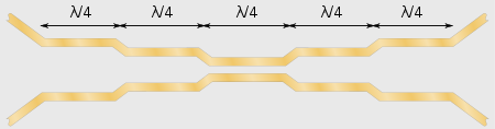Figure 8. A 5-section planar format directional coupler

It can be shown that coupled line directional couplers have $\tau \$ purely real and $\kappa \$ purely imaginary at all frequencies. This leads to a simplification of the S-matrix and the result that the coupled port is always in quadrature phase (90°) with the output port. Some applications make use of this phase difference. Letting $\kappa = i \kappa_\mathrm I \$, the ideal case of lossless operation simplifies to,^[19]

$\tau^2 + {\kappa_\mathrm I}^2 = 1 \$

Branch-line coupler

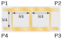Figure 9. A 3-section branch-line coupler implemented in planar format

The branch-line coupler consists of two parallel transmission lines physically coupled together with one or more branch lines between them. The branch lines are spaced λ/4 apart and represent sections of a multi-section filter design in the same way as the multiple sections of a coupled line coupler except that here the coupling of each section is controlled with the impedance of the branch lines. The main and coupled line are $\scriptstyle \sqrt 2$ of the system impedance. The more sections there are in the coupler, the higher is the ratio of impedances of the branch lines. High impedance lines have narrow tracks and this usually limits the design to three sections in planar formats due to manufacturing limitations. A similar limitation applies for coupling factors looser than 10 dB; low coupling also requires narrow tracks. Coupled lines are a better choice when loose coupling is required, but branch-line couplers are good for tight coupling and can be used for 3 dB hybrids. Branch-line couplers usually do not have such a wide bandwidth as coupled lines. This style of coupler is good for implementing in high-power, air dielectric, solid bar formats as the rigid structure is easy to mechanically support.^[20]

Lange coupler

The construction of the Lange coupler is similar to the interdigital filter with paralleled lines interleaved to achieve the coupling. It is used for strong couplings in the range 3 dB to 6 dB.^[21]

Power dividers

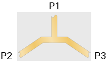Figure 10. Simple T-junction power division in planar format

The earliest transmission line power dividers were simple T-junctions. These suffer from very poor isolation between the output ports – a large part of the power reflected back from port 2 finds it way into port 3. It can be shown that it is not theoretically possible to simultaneously match all three ports of a passive, lossless three-port and poor isolation is unavoidable. It is, however, possible with four-ports and this is the fundamental reason why four-port devices are used to implement three-port power dividers: four-port devices can be designed so that power arriving at port 2 is split between port 1 and port 4 (which is terminated with a matching load) and none (in the ideal case) goes to port 3.^[22]

The term hybrid coupler originally applied to 3 dB coupled line directional couplers, that is, directional couplers in which the two outputs are each half the input power. This synonymously meant a quadrature 3 dB coupler with outputs 90° out of phase. Now any matched 4-port with isolated arms and equal power division is called a hybrid or hybrid coupler. Other types can have different phase relationships. If 90°, it is a 90° hybrid, if 180°, a 180° hybrid and so on. In this article hybrid coupler without qualification means a coupled line hybrid.^[23]

Wilkinson power divider

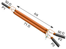Figure 11. Wilkinson divider in coaxial format

Main article: Wilkinson power divider

The Wilkinson power divider consists of two parallel uncoupled λ/4 transmission lines. The input is fed to both lines in parallel and the outputs are terminated with twice the system impedance bridged between them. The design can be realised in planar format but it has a more natural implementation in coax – in planar, the two lines have to be kept apart so they do not couple but have to be brought together at their outputs so they can be terminated whereas in coax the lines can be run side-by-side relying on the coax outer conductors for screening. The Wilkinson power divider solves the matching problem of the simple T-junction: it has low VSWR at all ports and high isolation between output ports. The input and output impedances at each port are designed to be equal to the characteristic impedance of the microwave system. This is achieved by making the line impedance $\scriptstyle \sqrt 2$ of the system impedance – for a 50 Ω system the Wilkinson lines are approximately 70 Ω^[24]

Hybrid coupler

Coupled line directional couplers are described above. When the coupling is designed to be 3 dB it is called a hybrid coupler. The S-matrix for an ideal, symmetric hybrid coupler reduces to;

$\mathbf S = \frac {1}{\sqrt 2} \begin{bmatrix} 0 & -i & -1 & 0 \\ -i & 0 & 0 & -1 \\ -1 & 0 & 0 & -i \\ 0 & -1 & -i & 0 \end{bmatrix}$

The two output ports have a 90° phase difference (-i to −1) and so this is a 90° hybrid.^[25]

Hybrid ring coupler

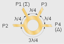Figure 12. Hybrid ring coupler in planar format

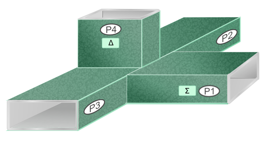
The hybrid ring coupler, also called the rat-race coupler, is a four-port 3 dB directional coupler consisting of a 3λ/2 ring of transmission line with four lines at the intervals shown in figure 12. Power input at port 1 splits and travels both ways round the ring. At ports 2 and 3 the signal arrives in phase and adds whereas at port 4 it is out of phase and cancels. Ports 2 and 3 are in phase with each other, hence this is an example of a 0° hybrid. Figure 12 shows a planar implementation but this design can also be implemented in coax or waveguide. Versions exist where each λ/4 section of the ring is alternately low and high impedance but a common compromise is to make the entire ring $\scriptstyle \sqrt 2$ of the port impedances – for a 50 Ω design the ring would be approximately 70 Ω.^[26]

The S-matrix for this hybrid is given by;

$\mathbf S = \frac {1}{\sqrt 2} \begin{bmatrix} 0 & -i & -i & 0 \\ -i & 0 & 0 & i \\ -i & 0 & 0 & -i \\ 0 & i & -i & 0 \end{bmatrix}$

The hybrid ring is not symmetric on its ports; choosing a different port as the input does not necessarily produce the same results. With port 1 or port 3 as the input the hybrid ring is a 0° hybrid as stated. However using port 2 or port 4 as the input results in a 180° hybrid.^[27] This fact leads to another useful application of the hybrid ring: it can be used to produce sum (Σ) and difference (Δ) signals from two input signals as shown in figure 12. With inputs to ports 2 and 3, the Σ signal appears at port 1 and the Δ signal appears at port 4.^[28]

Multiple output dividers

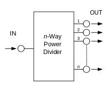Figure 13. Power Divider

A typical power divider is shown in figure 13. Ideally, input power would be divided equally between the output ports. Dividers are made up of multiple couplers and, like couplers, may be reversed and used as multiplexers. The drawback is that for a four channel multiplexer, the output consists of only 1/4 the power from each, and is relatively inefficient. The reason for this is that at each combiner half the input power goes to port 4 and is dissipated in the termination load. If the two inputs were coherent the phases could be so arranged that cancellation occurred at port 4 and then all the power would go to port 1. However, multiplexer inputs are usually from entirely independent sources and therefore not coherent. Lossless multiplexing can only be done with filter networks.^[29]

Waveguide types

Waveguide directional couplers

Waveguide branch-line coupler

The branch-line coupler described above can also be implemented in waveguide.^[30]

Bethe-hole directional coupler

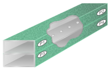Figure 14. A multi-hole directional coupler

One of the most common, and simplest, waveguide directional couplers is the Bethe-hole directional coupler. This consists of two parallel waveguides, one stacked on top of the other, with a hole between them. Some of the power from one guide is launched through the hole into the other. The Bethe-hole coupler is another example of a backward coupler.^[31]

The concept of the Bethe-hole coupler can be extended by providing multiple holes. The holes are spaced λ/4 apart. The design of such couplers has parallels with the multiple section coupled transmission lines. Using multiple holes allows the bandwidth to be extended by designing the sections as a Butterworth, Chebyshev, or some other filter class. The hole size is chosen to give the desired coupling for each section of the filter. Design criteria are to achieve a substantially flat coupling together with high directivity over the desired band.^[32]

Riblet short-slot coupler

The Riblet short-slot coupler is two waveguides side-by-side with the side-wall in common instead of the long side as in the Bethe-hole coupler. A slot is cut in the sidewall to allow coupling. This design is frequently used to produce a 3 dB coupler.^[33]

Schwinger reversed-phase coupler

The Schwinger reversed-phase coupler is another design using parallel waveguides, this time the long side of one is common with the short side-wall of the other. Two off-centre slots are cut between the waveguides spaced λ/4 apart. The Schwinger is a backward coupler. This design has the advantage of a substantially flat directivity response and the disadvantage of a strongly frequency-dependent coupling compared to the Bethe-hole coupler, which has little variation in coupling factor.^[34]

Moreno crossed-guide coupler

The Moreno crossed-guide coupler has two waveguides stacked one on top of the other like the Bethe-hole coupler but at right angles to each other instead of parallel. Two off-centre holes, usually cross-shaped are cut on the diagonal between the waveguides a distance $\scriptstyle \sqrt 2 \lambda / 4$ apart. The Moreno coupler is good for tight coupling applications. It is a compromise between the properties of the Bethe-hole and Schwinger couplers with both coupling and directivity varying with frequency.^[35]

Waveguide power dividers

Waveguide hybrid ring

The hybrid ring discussed above can also be implemented in waveguide.^[36]

Magic Tee

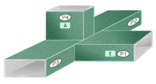Figure 15. Magic Tee

Main article: Magic Tee

Coherent power division was first accomplished by means of simple Tee junctions. At microwave frequencies, waveguide tees have two possible forms – the E-plane and H-plane. These two junctions split power equally, but because of the different field configurations at the junction, the electric fields at the output arms are in-phase for the H-plane tee and are anti-phase for the E-plane tee. The combination of these two tees to form a hybrid tee known as the Magic Tee. The Magic Tee is a four-port component which can perform the vector sum (Σ) and difference (Δ) of two coherent microwave signals.^[37]

Discrete element types

Hybrid transformer

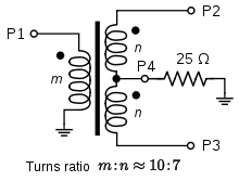Figure 16. 3 dB hybrid transformer for a 50 Ω system

Main article: Hybrid coil

The standard 3 dB hybrid transformer is shown in figure 16. Power at port 1 is split equally between ports 2 and 3 but in antiphase to each other. The hybrid transformer is therefore a 180° hybrid. The centre-tap is usually terminated internally but it is possible to bring it out as port 4; in which case the hybrid can be used as a sum and difference hybrid. However, port 4 presents as a different impedance to the other ports and will require an additional transformer for impedance conversion if it is required to use this port at the same sytem impedance.^[38]

Hybrid transformers are commonly used in telecommunications for 2 to 4 wire conversion. Telephone handsets include such a converter to convert the 2-wire line to the 4 wires from the earpiece and mouthpiece.^[39]

Cross-connected transformers

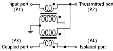Figure 17. Directional coupler using transformers

For lower frequencies (less than 600 MHz) a compact broadband implementation by means of RF transformers is possible. In figure 17 a circuit is shown which is meant for weak coupling and can be understood along these lines: A signal is coming in one line pair. One transformer reduces the voltage of the signal the other reduces the current. Therefore the impedance is matched. The same argument holds for every other direction of a signal through the coupler. The relative sign of the induced voltage and current determines the direction of the outgoing signal.^[40]

The coupling is given by;

$C_{3,1} = 20 \log n \$

where n is the secondary to primary turns ratio.

For a 3 dB coupling, that is equal splitting of the signal between the transmitted port and the coupled port, $\scriptstyle n = \sqrt 2$ and the isolated port is terminated in twice the characteristic impedance – 100 Ω for a 50 Ω system. A 3 dB power divider based on this circuit has the two outputs in 180° phase to each other, compared to λ/4 coupled lines which have a 90° phase relationship.^[41]

Resistive tee

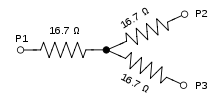Figure 18. Simple resistive tee circuit for a 50 Ω system

A simple tee circuit of resistors can be used as a power divider as shown in figure 18. This circuit can also be implemented as a delta circuit by applying the Y-Δ transform. The delta form uses resistors that are equal to the system impedance. This can be advantageous because precision resistors of the value of the system impedance are always available for most system nominal impedances. The tee cicuit has the benefits of simplicity and cheapness but has two major drawbacks. The first is that the circuit will dissipate power since it is resistive: an equal split will result in 6 dB insertion loss instead of 3 dB. The second problem is that there is 0 dB directivity leading to very poor isolation between the output ports.^[42]

The insertion loss is not such a problem for an unequal split of power: for instance -40 dB at port 3 has an insertion loss less than 0.2 dB at port 2. Isolation can be improved at the expense of insertion loss at both output ports by replacing the output resistors with T pads. The isolation improvement is greater than the insertion loss added.^[43]

6 dB resistive bridge hybrid

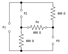Figure 19. 6 dB resistive bridge hybrid for a 600 Ω system

A true hybrid divider/coupler with, theoretically, infinite isolation and directivity can be made from a resistive bridge circuit. Like the tee circuit, the bridge has 6 dB insertion loss. It has the disadvantage that it cannot be used with unbalanced circuits without the addition of transformers; however, it is ideal for 600 Ω balanced telecommunication lines if the insertion loss is not an issue. The resistors in the bridge which represent ports are not usually part of the device (with the exception of port 4 which may well be left permanently terminatied internally) these being provided by the line terminations. The device thus consists essentially of two resistors (plus the port 4 termination).^[44]

Applications

Monitoring

The coupled output from the directional coupler can be used to monitor frequency and power level on the signal without interrupting the main power flow in the system (except for a power reduction – see figure 3).^[45]

Making use of isolation

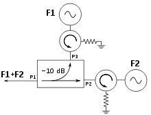Figure 20. Two-tone receiver test setup

If isolation is high, directional couplers are good for combining signals to feed a single line to a receiver for two-tone receiver tests. In figure 20, one signal enters port P₃ and one enters port P₂, while both exit port P₁. The signal from port P₃ to port P₁ will experience 10 dB of loss, and the signal from port P₂ to port P₁ will have 0.5 dB loss. The internal load on the isolated port will dissipate the signal losses from port P₃ and port P₂. If the isolators in figure 20 are neglected, the isolation measurement (port P₂ to port P₃) determines the amount of power from the signal generator F₂ that will be injected into the signal generator F₁. As the injection level increases, it may cause modulation of signal generator F₁, or even injection phase locking. Because of the symmetry of the directional coupler, the reverse injection will happen with the same possible modulation problems of signal generator F₂ by F₁. Therefore the isolators are used in figure 20 to effectively increase the isolation (or directivity) of the directional coupler. Consequently the injection loss will be the isolation of the directional coupler plus the reverse isolation of the isolator.^[46]

Hybrids

Applications of the hybrid include monopulse comparators, mixers, power combiners, dividers, modulators, and phased array radar antenna systems. Both in-phase devices (such as the Wilkinson divider) and quadrature (90°) hybrid couplers may be used for coherent power divider applications. An example of quadrature hybrids being used in a coherent power combiner application is given in the next section.^[47]

An inexpensive version of the power divider is used in the home to divide cable TV or over-the-air TV signals to multiple TV sets and other devices. Multiport splitters with more than two output ports usually consist internally of a number of cascaded couplers. Domestic broadband internet service can be provided by cable TV companies (cable internet). The domestic user's internet cable modem is connected to one port of the splitter.^[48]

Power combiners

Since hybrid circuits are bi-directional, they can be used to coherently combine power as well as splitting it. In figure 21, an example is shown of a signal split up to feed multiple low power amplifiers, then recombined to feed a single antenna with high power.^[49]

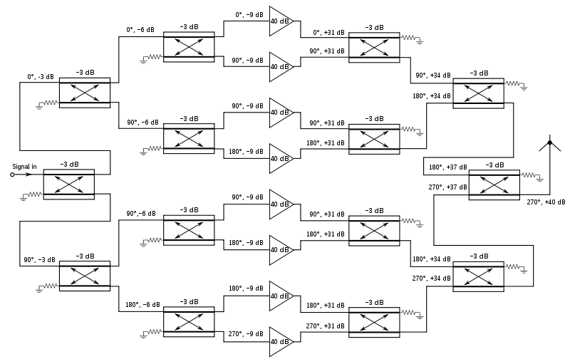Figure 21. Splitter and combiner networks used with amplifiers to produce a high power 40 dB (voltage gain 100) solid state amplifier

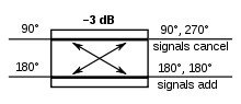Figure 22. Phase arrangement on a hybrid power combiner.

The phases of the inputs to each power combiner are arranged such that the two inputs are 90° out of phase with each other. Since the coupled port of a hybrid combiner is 90° out of phase with the transmitted port, this causes the powers to add at the output of the combiner and to cancel at the isolated port: a representative example from figure 21 is shown in figure 22. Note that there is an additional fixed 90° phase shift to both ports at each combiner/divider which is not shown in the diagrams for simplicity.^[50] Applying in-phase power to both input ports would not get the desired result: the quadrature sum of the two inputs would appear at both output ports – that is half the total power out of each. This approach allows the use of numerous less expensive and lower-power amplifiers in the circuitry instead of a single high-power TWT. Yet another approach is to have each solid state amplifier (SSA) feed an antenna and let the power be combined in space or be used to feed a lens attached to an antenna.^[51]

Phase difference

Figure 23. Phase combination of two antennae

The phase properties of a 90° hybrid coupler can be used to great advantage in microwave circuits. For example in a balanced microwave amplifier the two input stages are fed through a hybrid coupler. The FET device normally has a very poor match and reflects much of the incident energy. However, since the devices are essentially identical the reflection coefficients from each device are equal. The reflected voltage from the FETs are in phase at the isolated port and are 180° different at the input port. Therefore, all of the reflected power from the FETs goes to the load at the isolated port and no power goes to the input port. This results in a good input match (low VSWR).^[52]

If phase-matched lines are used for an antenna input to a 180° hybrid coupler as shown in figure 23, a null will occur directly between the antennas. To receive a signal in that position, one would have to either change the hybrid type or line length. To reject a signal from a given direction, or create the difference pattern for a monopulse radar, this is a good approach.^[53]

Phase-difference couplers can be used to create beam tilt in a VHF FM radio station, by delaying the phase to the lower elements of an antenna array. More generally, phase-difference couplers, together with fixed phase delays and antenna arrays, are used in beam-forming networks such as the Butler matrix, to create a radio beam in any prescribed direction.^[54]

See also

• Star coupler

References

1. ^ Ishii, p.200
   Naval Air Warfare Center, p.6-4.1
2. ^ Räisänen and Lehto, p.116
3. ^ Naval Air Warfare Center, p.6.4.1
4. ^ For instance; Morgan, p.149
5. ^ Naval Air Warfare Center, p.6.4.1
   Vizmuller, p.101
6. ^ Naval Air Warfare Center, p.6.4.2
7. ^ Naval Air Warfare Center, p.6.4.2
8. ^ Naval Air Warfare Center, p.6.4.3
9. ^ Dyer, p.479
   Ishii, p.216
   Räisänen and Lehto, pp.120–122
10. ^ For instance, Räisänen and Lehto, pp.120–122
11. ^ Naval Air Warfare Center, p.6.4.3
12. ^ Naval Air Warfare Center, p.6.4.3
13. ^ Morgan, p.149
    Matthaei et al., pp.775–777
    Vizmuller, p.101
14. ^ Naval Air Warfare Center, p.6.4.1
15. ^ Naval Air Warfare Center, p.6.4.1
    Matthaei et al., pp.585–588, 776–778
16. ^ Räisänen and Lehto, pp.124–126
    Vizmuller, pp.102–103
17. ^ Naval Air Warfare Center, p.6.4.1
18. ^ Naval Air Warfare Center, p.6.4.1
    Matthaei et al., pp.775–777
19. ^ Ishii, p.216
    Räisänen and Lehto, p.120-122
20. ^ Ishii, pp.223–226
    Matthaei et al., pp.809–811
    Räisänen and Lehto, p.127
21. ^ Räisänen and Lehto, p.126
22. ^ Räisänen and Lehto, pp.117–118
23. ^ Naval Air Warfare Center, pp.6.4.1, 6.4.3
24. ^ Dyer, p.480
    Räisänen and Lehto, p.118-119
    Naval Air Warfare Center, p.6.4.4
25. ^ Ishii, p.200
26. ^ Ishii, pp. 229–230
    Morgan, p. 150
    Räisänen and Lehto, pp. 126–127
27. ^ Ishii, p. 201
28. ^ Räisänen and Lehto, pp. 122, 127
29. ^ Reddy et al., pp.60, 71
    Naval Air Warfare Center, pp.6.4.4, 6.4.5
30. ^ Matthaei et al., pp.811–812
    Ishii, pp.223–226
31. ^ Ishii, p.202
    Morgan, p.149
32. ^ Ishii, pp.205–6, 209
    Morgan, p.149
    Räisänen and Lehto, pp.122–123
33. ^ Ishii, p.211
34. ^ Ishii, pp.211–212
35. ^ Ishii, pp.212–213
36. ^ Morgan, p.149
37. ^ Naval Air Warfare Center, p.6.4.4
    Ishii, p.201
    Räisänen and Lehto, pp.123–124
38. ^ Hickman, pp.50–51
39. ^ Bigelow et al., p.211
    Chapuis and Joel, p.512
40. ^ Vizmuller, pp.107–108
41. ^ Vizmuller, p.108
42. ^ Hickman, pp.49–50
43. ^ Hickman, p.50
44. ^ Bryant, pp.114–115
45. ^ Naval Air Warfare Center, p.6.4.1
46. ^ Naval Air Warfare Center, pp.6.4.2–6.4.3
47. ^ Naval Air Warfare Center, pp.6.4.3–6.4.4
48. ^ Chen, p.76
    Gralla, pp.61-62
49. ^ Räisänen and Lehto, p.116
50. ^ Ishii, p.200
51. ^ Naval Air Warfare Center, p.6.4.5
52. ^ Naval Air Warfare Center, p.6.4.3
53. ^ Naval Air Warfare Center, p.6.4.4
54. ^ Fujimoto, pp.199–201
    Lo and Lee, p.27.7

Bibliography

 This article incorporates public domain material from the Avionics Department of the Naval Air Warfare Center Weapons Division document "Electronic Warfare and Radar Systems Engineering Handbook (report number TS 92-78)" (retrieved on 9 June 2006) (pp 6–4.1 to 6–4.5 Power Dividers and Directional Couplers).

• Stephen J. Bigelow, Joseph J. Carr, Steve Winder, Understanding telephone electronics Newnes, 2001 ISBN 0750671750.
• Geoff H. Bryant, Principles of Microwave Measurements, Institution of Electrical Engineers, 1993 ISBN 0863412963.
• Robert J. Chapuis, Amos E. Joel, 100 Years of Telephone Switching (1878–1978): Electronics, computers, and telephone switching (1960–1985), IOS Press, 2003 ISBN 1586033727.
• Walter Y. Chen, Home Networking Basis, Prentice Hall Professional, 2003 ISBN 0130165115.
• Stephen A. Dyer, Survey of instrumentation and measurement Wiley-IEEE, 2001 ISBN 047139484X.
• Kyōhei Fujimoto, Mobile Antenna Systems Handbook, Artech House, 2008 ISBN 1596931264.
• Preston Gralla, How the Internet Works, Que Publishing, 1998 ISBN 0789717263.
• Ian Hickman, Practical Radio-frequency Handbook, Newnes, 2006 ISBN 0750680393.
• Thomas Koryu Ishii, Handbook of Microwave Technology: Components and devices, Academic Press, 1995 ISBN 0123746965.
• Y. T. Lo, S. W. Lee, Antenna Handbook: Applications, Springer, 1993 ISBN 0442015941.
• Matthaei, George L.; Young, Leo and Jones, E. M. T. Microwave Filters, Impedance-Matching Networks, and Coupling Structures McGraw-Hill 1964 OCLC 299575271
• D. Morgan, A Handbook for EMC Testing and Measurement, IET, 1994 ISBN 0863417566.
• Antti V. Räisänen, Arto Lehto, Radio engineering for wireless communication and sensor applications, Artech House, 2003 ISBN 1580535429.
• K.R. Reddy, S. B. Badami, V. Balasubramanian, Oscillations And Waves, Universities Press, 1994 ISBN 817371018X.
• Peter Vizmuller, RF design guide: systems, circuits, and equations, Volume 1, Artech House, 1995 ISBN 0890067546.