Atmospheric model

A 96-hour forecast of 850 mbar geopotential height and temperature from the Global Forecast System

An atmospheric model is a mathematical model constructed around the full set of primitive dynamical equations which govern atmospheric motions. It can supplement these equations with parameterizations for turbulent diffusion, radiation, moist processes (clouds and precipitation), heat exchange, soil, vegetation, surface water, the kinematic effects of terrain, and convection. Most atmospheric models are numerical, i.e. they discretize equations of motion. They can predict microscale phenomena such as tornadoes and boundary layer eddies, sub-microscale turbulent flow over buildings, as well as synoptic and global flows. The horizontal domain of a model is either global, covering the entire Earth, or regional (limited-area), covering only part of the Earth. The different types of models run are thermotropic, barotropic, hydrostatic, and nonhydrostatic. Some of the model types make assumptions about the atmosphere which lengthens the time steps used and increases computational speed.

Forecasts are computed using mathematical equations for the physics and dynamics of the atmosphere. These equations are nonlinear and are impossible to solve exactly. Therefore, numerical methods obtain approximate solutions. Different models use different solution methods. Global models often use spectral methods for the horizontal dimensions and finite-difference methods for the vertical dimension, while regional models usually use finite-difference methods in all three dimensions. For specific locations, model output statistics use climate information, output from numerical weather prediction, and current surface weather observations to develop statistical relationships which account for model bias and resolution issues.

Types

The main assumption made by the thermotropic model is that while the magnitude of the thermal wind may change, its direction does not change with respect to height, and thus the baroclinicity in the atmosphere can be simulated using the 500 mb (15 inHg) and 1,000 mb (30 inHg) geopotential height surfaces and the average thermal wind between them.^[1][2]

Barotropic models assume the atmosphere is nearly barotropic, which means that the direction and speed of the geostrophic wind are independent of height. In other words, no vertical wind shear of the geostrophic wind. It also implies that thickness contours (a proxy for temperature) are parallel to upper level height contours. In this type of atmosphere, high and low pressure areas are centers of warm and cold temperature anomalies. Warm-core highs (such as the subtropical ridge and Bermuda-Azores high) and cold-core lows have strengthening winds with height, with the reverse true for cold-core highs (shallow arctic highs) and warm-core lows (such as tropical cyclones).^[3] A barotropic model tries to solve a simplified form of atmospheric dynamics based on the assumption that the atmosphere is in geostrophic balance; that is, that the Rossby number of the air in the atmosphere is small.^[4] If the assumption is made that the atmosphere is divergence-free, the curl of the Euler equations reduces into the barotropic vorticity equation. This latter equation can be solved over a single layer of the atmosphere. Since the atmosphere at a height of approximately 5.5 kilometres (3.4 mi) is mostly divergence-free, the barotropic model best approximates the state of the atmosphere at a geopotential height corresponding to that altitude, which corresponds to the atmosphere's 500 mb (15 inHg) pressure surface.^[5]

Hydrostatic models filter out vertically moving acoustic waves from the vertical momentum equation, which significantly increases the time step used within the model's run. This is known as the hydrostatic approximation. Hydrostatic models use either pressure or sigma-pressure vertical coordinates. Pressure coordinates intersect topography while sigma coordinates follow the contour of the land. Its hydrostatic assumption is reasonable as long as horizontal grid resolution is not small, which is a scale where the hydrostatic assumption fails. Models which use the entire vertical momentum equation are known as nonhydrostatic. A nonhydrostatic model can be solved anelastically, meaning it solves the complete continuity equation for air, or elastically, meaning it solves the complete continuity equation for air and is fully compressible. Nonhydrostatic models use altitude or sigma altitude for their vertical coordinates. Altitude coordinates can intersect land while sigma-altitude coordinates follow the contours of the land.^[6]

History

The ENIAC main control panel at the Moore School of Electrical Engineering

Main article: History of numerical weather prediction

The history of numerical weather prediction began in the 1920s through the efforts of Lewis Fry Richardson who utilized procedures developed by Vilhelm Bjerknes.^[7][8] It was not until the advent of the computer and computer simulation that computation time was reduced to less than the forecast period itself. ENIAC created the first computer forecasts in 1950,^[5][9] and more powerful computers later increased the size of initial datasets and included more complicated versions of the equations of motion.^[10] In 1966, West Germany and the United States began producing operational forecasts based on primitive-equation models, followed by the United Kingdom in 1972 and Australia in 1977.^[7][11] The development of global forecasting models led to the first climate models.^[12][13] The development of limited area (regional) models facilitated advances in forecasting the tracks of tropical cyclone as well as air quality in the 1970s and 1980s.^[14][15]

Because the output of forecast models based on atmospheric dynamics requires corrections near ground level, model output statistics (MOS) were developed in the 1970s and 1980s for individual forecast points (locations).^[16][17] Even with the increasing power of supercomputers, the forecast skill of numerical weather models only extends to about two weeks into the future, since the density and quality of observations—together with the chaotic nature of the partial differential equations used to calculate the forecast—introduce errors which double every five days.^[18][19] The use of model ensemble forecasts since the 1990s helps to define the forecast uncertainty and extend weather forecasting farther into the future than otherwise possible.^[20][21][22]

Initialization

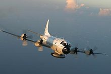A WP-3D Orion weather reconnaissance aircraft in flight

The atmosphere is a fluid. As such, the idea of numerical weather prediction is to sample the state of the fluid at a given time and use the equations of fluid dynamics and thermodynamics to estimate the state of the fluid at some time in the future. On land, terrain maps, available at resolutions down to 1 kilometre (0.62 mi) globally, are used to help model atmospheric circulations within regions of rugged topography, in order to better depict features such as downslope winds, mountain waves, and related cloudiness which affects incoming solar radiation.^[23] The main inputs from country-based weather services are surface observations from automated weather stations at ground level over land and from weather buoys at sea. The World Meteorological Organization acts to standardize the instrumentation, observing practices and timing of these observations worldwide. Stations either report hourly in METAR reports,^[24] or every six hours in SYNOP reports.^[25] Models are initialized using this observed data. The irregularly spaced observations are processed by data assimilation and objective analysis methods, which perform quality control and obtain values at locations usable by the model's mathematical algorithms. The grid used for global models is geodesic or icosahedral, spaced by latitude, longitude, and elevation.^[26] The data are then used in the model as the starting point for a forecast.^[27]

A variety of methods are used to gather observational data for use in numerical models. Sites launch radiosondes, which rise through the troposphere and well into the stratosphere.^[28] Information from weather satellites is used where traditional data sources are not available. Commerce provides pilot reports along aircraft routes^[29] and ship reports along shipping routes.^[30] Research projects use reconnaissance aircraft to fly in and around weather systems of interest, such as tropical cyclones.^[31][32] Reconnaissance aircraft are also flown over the open oceans during the cold season into systems which cause significant uncertainty in forecast guidance, or are expected to be of high impact 3–7 days into the future over the downstream continent.^[33] Sea ice began to be initialized in forecast models in 1971.^[34] Efforts to involve sea surface temperature in model initialization began in 1972 due to its role in modulating weather in higher latitudes of the Pacific.^[35]

Computation

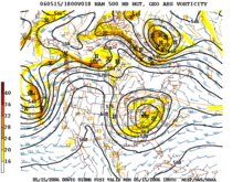An example of 500 mbar geopotential height prediction from a numerical weather prediction model.

Supercomputers are capable of running highly complex models to help scientists better understand Earth's climate.

A model is a computer program that produces meteorological information for future times at given locations and altitudes. Within any model is a set of equations, known as the primitive equations, used to predict the future state of the atmosphere.^[36] These equations are initialized from the analysis data and rates of change are determined. These rates of change predict the state of the atmosphere a short time into the future, with each time increment known as a time step. The equations are then applied to this new atmospheric state to find new rates of change, and these new rates of change predict the atmosphere at a yet further time into the future. Time stepping is repeated until the solution reaches the desired forecast time. The length of the time step chosen within the model is related to the distance between the points on the computational grid, and is chosen to maintain numerical stability.^[37] Time steps for global models are on the order of tens of minutes,^[38] while time steps for regional models are between one and four minutes.^[39] The global models are run at varying times into the future. The UKMET Unified model is run six days into the future,^[40] the European Centre for Medium-Range Weather Forecasts model is run out to 10 days into the future,^[41] while the Global Forecast System model run by the Environmental Modeling Center is run 16 days into the future.^[42]

The equations used are nonlinear partial differential equations which are impossible to solve exactly through analytical methods,^[43] with the exception of a few idealized cases.^[44] Therefore, numerical methods obtain approximate solutions. Different models use different solution methods: some global models use spectral methods for the horizontal dimensions and finite difference methods for the vertical dimension, while regional models and other global models usually use finite-difference methods in all three dimensions.^[43] The visual output produced by a model solution is known as a prognostic chart, or prog.^[45]

Parameterization

Weather and climate model gridboxes have sides of between 5 kilometres (3.1 mi) and 300 kilometres (190 mi). A typical cumulus cloud has a scale of less than 1 kilometre (0.62 mi), and would require a grid even finer than this to be represented physically by the equations of fluid motion. Therefore the processes that such clouds represent are parameterized, by processes of various sophistication. In the earliest models, if a column of air in a model gridbox was unstable (i.e., the bottom warmer than the top) then it would be overturned, and the air in that vertical column mixed. More sophisticated schemes add enhancements, recognizing that only some portions of the box might convect and that entrainment and other processes occur. Weather models that have gridboxes with sides between 5 kilometres (3.1 mi) and 25 kilometres (16 mi) can explicitly represent convective clouds, although they still need to parameterize cloud microphysics.^[46] The formation of large-scale (stratus-type) clouds is more physically based, they form when the relative humidity reaches some prescribed value. Still, sub grid scale processes need to be taken into account. Rather than assuming that clouds form at 100% relative humidity, the cloud fraction can be related to a critical relative humidity of 70% for stratus-type clouds, and at or above 80% for cumuliform clouds,^[47] reflecting the sub grid scale variation that would occur in the real world.

The amount of solar radiation reaching ground level in rugged terrain, or due to variable cloudiness, is parameterized as this process occurs on the molecular scale.^[48] Also, the grid size of the models is large when compared to the actual size and roughness of clouds and topography. Sun angle as well as the impact of multiple cloud layers is taken into account.^[49] Soil type, vegetation type, and soil moisture all determine how much radiation goes into warming and how much moisture is drawn up into the adjacent atmosphere. Thus, they are important to parameterize.^[50]

Domains

The horizontal domain of a model is either global, covering the entire Earth, or regional, covering only part of the Earth. Regional models also are known as limited-area models, or LAMs. Regional models use finer grid spacing to resolve explicitly smaller-scale meteorological phenomena, since their smaller domain decreases computational demands. Regional models use a compatible global model for initial conditions of the edge of their domain. Uncertainty and errors within LAMs are introduced by the global model used for the boundary conditions of the edge of the regional model, as well as within the creation of the boundary conditions for the LAMs itself.^[51]

The vertical coordinate is handled in various ways. Some models, such as Richardson's 1922 model, use geometric height (z) as the vertical coordinate. Later models substituted the geometric z coordinate with a pressure coordinate system, in which the geopotential heights of constant-pressure surfaces become dependent variables, greatly simplifying the primitive equations.^[52] This follows since pressure decreases with height through the Earth's atmosphere.^[53] The first model used for operational forecasts, the single-layer barotropic model, used a single pressure coordinate at the 500-millibar (15 inHg) level,^[5] and thus was essentially two-dimensional. High-resolution models—also called mesoscale models—such as the Weather Research and Forecasting model tend to use normalized pressure coordinates referred to as sigma coordinates.^[54] This coordinate system receives that name since the independent variable σ is used to represent a pressure level (p) scaled with the surface pressure (p₀) and in some cases the pressure at the top of the domain (p_T).^[55]

Global versions

Some of the better known global numerical models are:

• GFS Global Forecast System (previously AVN) – developed by NOAA
• NOGAPS – developed by the US Navy to compare with the GFS
• GEM Global Environmental Multiscale Model – developed by the Meteorological Service of Canada (MSC)
• IFS developed by the European Centre for Medium-Range Weather Forecasts
• UM Unified Model developed by the UK Met Office, but is hand-corrected by professional forecasters
• GME developed by the German Weather Service, DWD, NWP Global model of DWD
• ARPEGE developed by the French Weather Service, Météo-France
• IGCM Intermediate General Circulation Model^[40]

Regional versions

Some of the better known regional numerical models are:

• WRF The Weather Research and Forecasting model was developed cooperatively by NCEP, NCAR, and the meteorological research community. WRF has several configurations, including:

• WRF-NMM The WRF Nonhydrostatic Mesoscale Model is the primary short-term weather forecast model for the U.S., replacing the Eta model.
• AR-WRF Advanced Research WRF developed primarily at the U.S. National Center for Atmospheric Research (NCAR)

• NAM The term North American Mesoscale model refers to whatever regional model NCEP operates over the North American domain. NCEP began using this designation system in January 2005. Between January 2005 and May 2006 the Eta model used this designation. Beginning in May 2006, NCEP began to use the WRF-NMM as the operational NAM.
• RAMS the Regional Atmospheric Modeling System developed at Colorado State University for numerical simulations of atmospheric meteorology and other environmental phenomena on scales from meters to hundreds of kilometers - now supported in the public domain
• MM5 The Fifth Generation Penn State/NCAR Mesoscale Model
• ARPS the Advanced Region Prediction System developed at the University of Oklahoma is a comprehensive multi-scale nonhydrostatic simulation and prediction system that can be used for regional-scale weather prediction up to the tornado-scale simulation and prediction. Advanced radar data assimilation for thunderstorm prediction is a key part of the system..
• HIRLAM High Resolution Limited Area Model
• GEM-LAM Global Environmental Multiscale Limited Area Model, the high resolution (2.5 km) GEM by the Meteorological Service of Canada (MSC)
• ALADIN The high-resolution limited-area hydrostatic and non-hydrostatic model developed and operated by several European and North African countries under the leadership of Météo-France^[40]
• COSMO The COSMO Model, formerly known as LM, aLMo or LAMI, is a limited-area non-hydrostatic model developed within the framework of the Consortium for Small-Scale Modelling (Germany, Switzerland, Italy, Greece, Poland, Romania, and Russia).^[56]

1. COSMO The COSMO Model (formerly known as LM, aLMo or LAMI) is a limited-area non-hydrostatic model for operational numerical weather prediction, regional climate modelling, environmental prediction (aerosols, pollen and atmospheric chemistry) and research (idealised case studies). A first NWP version was originally developed by the German Weather Service. It is now further developed by the Consortium for Small-Scale Modelling, the Climate Limited-area Modelling (CLM)-Community, and other research institutes.[1]

Model output statistics

Main article: Model output statistics

Because forecast models based upon the equations for atmospheric dynamics do not perfectly determine weather conditions near the ground, statistical corrections were developed to attempt to resolve this problem. Statistical models were created based upon the three-dimensional fields produced by numerical weather models, surface observations, and the climatological conditions for specific locations. These statistical models are collectively referred to as model output statistics (MOS),^[57] and were developed by the National Weather Service for their suite of weather forecasting models.^[16] The United States Air Force developed its own set of MOS based upon their dynamical weather model by 1983.^[17]

Model output statistics differ from the perfect prog technique, which assumes that the output of numerical weather prediction guidance is perfect.^[58] MOS can correct for local effects that cannot be resolved by the model due to insufficient grid resolution, as well as model biases. Forecast parameters within MOS include maximum and minimum temperatures, percentage chance of rain within a several hour period, precipitation amount expected, chance that the precipitation will be frozen in nature, chance for thunderstorms, cloudiness, and surface winds.^[59]

Applications

Climate modeling

See also: Global climate model

In 1956, Norman Phillips developed a mathematical model which could realistically depict monthly and seasonal patterns in the troposphere; this became the first successful climate model.^[12][13] Following Phillips's work, several groups began working to create general circulation models.^[60] The first general circulation climate model that combined both oceanic and atmospheric processes was developed in the late 1960s at the NOAA Geophysical Fluid Dynamics Laboratory.^[61] By the early 1980s, the United States' National Center for Atmospheric Research had developed the Community Atmosphere Model; this model has been continuously refined into the 2000s.^[62] In 1986, efforts began to initialize and model soil and vegetation types, which led to more realistic forecasts.^[63] Coupled ocean-atmosphere climate models such as the Hadley Centre for Climate Prediction and Research's HadCM3 model are currently being used as inputs for climate change studies.^[60]

Limited area modeling

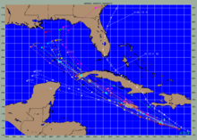Model spread with Hurricane Ernesto (2006) within the National Hurricane Center limited area models

See also: Tropical cyclone forecast model

Air quality forecasts depend on Atmospheric models to provide fluid flow information for tracking the movement of a pollutant.^[64] The Urban Airshed Model, a regional forecast model for the effects of air pollution and acid rain, was developed by a private company in the USA in 1970. Development of this model was taken over by the Environmental Protection Agency and improved in the mid to late 1970s using results from a regional air pollution study. While developed in California, this model was later used in other areas of North America, Europe and Asia during the 1980s.^[15]

In 1978, the first hurricane-tracking model based on atmospheric dynamics – the movable fine-mesh (MFM) model – began operating.^[14] Within the field of tropical cyclone track forecasting, despite the ever-improving dynamical model guidance which occurred with increased computational power, it was not until the decade of the 1980s when numerical weather prediction showed skill, and until the 1990s when it consistently outperformed statistical or simple dynamical models.^[65] However, predictions of the intensity of a tropical cyclone based on numerical weather prediction continues to be a challenge, since statical methods continue to show higher skill over dynamical guidance.^[66]

See also

• Climate model
• Numerical weather prediction
• Upper Atmospheric Models

References

1. ^ Gates, W. Lawrence (August 1955). Results Of Numerical Forecasting With The Barotropic And Thermotropic Atmospheric Models. Hanscom Air Force Base: Air Force Cambridge Research Laboratories. http://handle.dtic.mil/100.2/AD101943. Retrieved 2011-02-11. 
2. ^ Thompson, P. D.; W. Lawrence Gates (April 1956). "A Test of Numerical Prediction Methods Based on the Barotropic and Two-Parameter Baroclinic Models". Journal of Meteorology 13 (2): 127–141. Bibcode 1956JAtS...13..127T. doi:10.1175/1520-0469(1956)013<0127:ATONPM>2.0.CO;2. ISSN 1520-0469. 
3. ^ Wallace, John M. and Peter V. Hobbs (1977). Atmospheric Science: An Introductory Survey. Academic Press, Inc.. pp. 384–385. ISBN 0127329501. 
4. ^ Marshall, John; Plumb, R. Alan (2008). "Balanced flow". Atmosphere, ocean, and climate dynamics : an introductory text. Amsterdam: Elsevier Academic Press. pp. 109–12. ISBN 9780125586917. 
5. ^ ^{a b c} Charney, Jule; Fjörtoft, Ragnar; von Neumann, John (November 1950). "Numerical Integration of the Barotropic Vorticity Equation". Tellus 2 (4): 237–254. Bibcode 1950Tell....2..237C. doi:10.1111/j.2153-3490.1950.tb00336.x. 
6. ^ Jacobson, Mark Zachary (2005). Fundamentals of atmospheric modeling. Cambridge University Press. pp. 138–143. ISBN 9780521839709. http://books.google.com/?id=WPwEf-1f73wC&pg=PA139&lpg=PA139&dq=hydrostatic+model+book#v=onepage&q=hydrostatic%20model%20book&f=false. Retrieved 2011-02-15. 
7. ^ ^{a b} Lynch, Peter (2008-03-20). "The origins of computer weather prediction and climate modeling". Journal of Computational Physics (University of Miami) 227 (7): 3431–44. Bibcode 2008JCoPh.227.3431L. doi:10.1016/j.jcp.2007.02.034. http://www.rsmas.miami.edu/personal/miskandarani/Courses/MPO662/Lynch,Peter/OriginsCompWF.JCP227.pdf. Retrieved 2010-12-23. 
8. ^ Lynch, Peter (2006). "Weather Prediction by Numerical Process". The Emergence of Numerical Weather Prediction. Cambridge University Press. pp. 1–27. ISBN 9780521857291. 
9. ^ Cox, John D. (2002). Storm Watchers. John Wiley & Sons, Inc.. p. 208. ISBN 047138108X. 
10. ^ Harper, Kristine; Uccellini, Louis W.; Kalnay, Eugenia; Carey, Kenneth; Morone, Lauren (May 2007). "2007: 50th Anniversary of Operational Numerical Weather Prediction". Bulletin of the American Meteorological Society 88 (5): 639–650. Bibcode 2007BAMS...88..639H. doi:10.1175/BAMS-88-5-639. 
11. ^ Leslie, L.M.; Dietachmeyer, G.S. (December 1992). "Real-time limited area numerical weather prediction in Australia: a historical perspective". Australian Meteorological Magazine (Bureau of Meteorology) 41 (SP): 61–77. http://www.bom.gov.au/amoj/docs/1992/leslie2.pdf. Retrieved 2011-01-03. 
12. ^ ^{a b} Phillips, Norman A. (April 1956). "The general circulation of the atmosphere: a numerical experiment". Quarterly Journal of the Royal Meteorological Society 82 (352): 123–154. Bibcode 1956QJRMS..82..123P. doi:10.1002/qj.49708235202. 
13. ^ ^{a b} Cox, John D. (2002). Storm Watchers. John Wiley & Sons, Inc.. p. 210. ISBN 047138108X. 
14. ^ ^{a b} Shuman, Frederick G. (September 1989). "History of Numerical Weather Prediction at the National Meteorological Center". Weather and Forecasting 4 (3): 286–296. Bibcode 1989WtFor...4..286S. doi:10.1175/1520-0434(1989)004<0286:HONWPA>2.0.CO;2. ISSN 1520-0434. 
15. ^ ^{a b} Steyn, D. G. (1991). Air pollution modeling and its application VIII, Volume 8. Birkhäuser. pp. 241–242. ISBN 9780306438288. 
16. ^ ^{a b} Harry Hughes (1976). Model output statistics forecast guidance. United States Air Force Environmental Technical Applications Center. pp. 1–16. 
17. ^ ^{a b} L. Best, D. L. and S. P. Pryor (1983). Air Weather Service Model Output Statistics Systems. Air Force Global Weather Central. pp. 1–90. 
18. ^ Cox, John D. (2002). Storm Watchers. John Wiley & Sons, Inc.. pp. 222–224. ISBN 047138108X. 
19. ^ Weickmann, Klaus, Jeff Whitaker, Andres Roubicek and Catherine Smith (2001-12-01). The Use of Ensemble Forecasts to Produce Improved Medium Range (3–15 days) Weather Forecasts. Climate Diagnostics Center. Retrieved 2007-02-16.
20. ^ Toth, Zoltan; Kalnay, Eugenia (December 1997). "Ensemble Forecasting at NCEP and the Breeding Method". Monthly Weather Review 125 (12): 3297–3319. Bibcode 1997MWRv..125.3297T. doi:10.1175/1520-0493(1997)125<3297:EFANAT>2.0.CO;2. ISSN 1520-0493. 
21. ^ "The Ensemble Prediction System (EPS)". ECMWF. http://www.ecmwf.int/products/forecasts/guide/The_Ensemble_Prediction_System_EPS_1.html. Retrieved 2011-01-05. 
22. ^ Molteni, F.; Buizza, R.; Palmer, T.N.; Petroliagis, T. (January 1996). "The ECMWF Ensemble Prediction System: Methodology and validation". Quarterly Journal of the Royal Meteorological Society 122 (529): 73–119. Bibcode 1996QJRMS.122...73M. doi:10.1002/qj.49712252905. 
23. ^ Stensrud, David J. (2007). Parameterization schemes: keys to understanding numerical weather prediction models. Cambridge University Press. p. 56. ISBN 9780521865401. http://books.google.com/?id=lMXSpRwKNO8C&pg=PA56&dq=radiation+mountain+parameterization+book#v=onepage&q=radiation%20mountain%20parameterization%20book&f=false. Retrieved 2011-02-15. 
24. ^ National Climatic Data Center (2008-08-20). "Key to METAR Surface Weather Observations". National Oceanic and Atmospheric Administration. http://www.ncdc.noaa.gov/oa/climate/conversion/swometardecoder.html. Retrieved 2011-02-11. 
25. ^ "SYNOP Data Format (FM-12): Surface Synoptic Observations". UNISYS. 2008-05-25. Archived from the original on 2007-12-30. http://web.archive.org/web/20071230100059/http://weather.unisys.com/wxp/Appendices/Formats/SYNOP.html. 
26. ^ Kwon, J. H. (2007). Parallel computational fluid dynamics: parallel computings and its applications : proceedings of the Parallel CFD 2006 Conference, Busan city, Korea (May 15–18, 2006). Elsevier. p. 224. ISBN 9780444530356. http://books.google.com/?id=BQ_7vh5SrHQC&pg=PA224&dq=geodesic+grid+numerical+weather+prediction+book#v=onepage&q=geodesic%20grid%20numerical%20weather%20prediction%20book&f=false. Retrieved 2011-01-06. 
27. ^ "The WRF Variational Data Assimilation System (WRF-Var)". University Corporation for Atmospheric Research. 2007-08-14. Archived from the original on 2007-08-14. http://web.archive.org/web/20070814044336/http://www.mmm.ucar.edu/wrf/WG4/wrfvar/wrfvar-tutorial.htm. 
28. ^ Gaffen, Dian J. (2007-06-07). "Radiosonde Observations and Their Use in SPARC-Related Investigations". Archived from the original on 2007-06-07. http://web.archive.org/web/20070607142822/http://www.aero.jussieu.fr/~sparc/News12/Radiosondes.html. 
29. ^ Ballish, Bradley A. and V. Krishna Kumar (2008-05-23). Investigation of Systematic Differences in Aircraft and Radiosonde Temperatures with Implications for NWP and Climate Studies. Retrieved 2008-05-25.
30. ^ National Data Buoy Center (2009-01-28). "The WMO Voluntary Observing Ships (VOS) Scheme". National Oceanic and Atmospheric Administration. http://www.vos.noaa.gov/vos_scheme.shtml. Retrieved 2011-02-15. 
31. ^ 403rd Wing (2011). "The Hurricane Hunters". 53rd Weather Reconnaissance Squadron. http://www.hurricanehunters.com. Retrieved 2006-03-30. 
32. ^ Lee, Christopher (2007-10-08). "Drone, Sensors May Open Path Into Eye of Storm". The Washington Post. http://www.washingtonpost.com/wp-dyn/content/article/2007/10/07/AR2007100700971_pf.html. Retrieved 2008-02-22. 
33. ^ National Oceanic and Atmospheric Administration (2010-11-12). "NOAA Dispatches High-Tech Research Plane to Improve Winter Storm Forecasts". http://www.noaanews.noaa.gov/stories2010/20100112_plane.html. Retrieved 2010-12-22. 
34. ^ Stensrud, David J. (2007). Parameterization schemes: keys to understanding numerical weather prediction models. Cambridge University Press. p. 137. ISBN 9780521865401. http://books.google.com/?id=lMXSpRwKNO8C&pg=PA137&dq=sea+ice+use+numerical+weather+prediction+book#v=onepage&q=sea%20ice%20use%20numerical%20weather%20prediction%20book&f=false. Retrieved 2011-01-08. 
35. ^ Houghton, John Theodore (1985). The Global Climate. Cambridge University Press archive. pp. 49–50. ISBN 9780521312561. http://books.google.com/?id=SV04AAAAIAAJ&pg=PA38&dq=sea+surface+temperature+importance+use+numerical+weather+prediction+book#v=onepage&q=sea%20surface%20temperature%20importance%20use%20numerical%20weather%20prediction%20book&f=false. Retrieved 2011-01-08. 
36. ^ Pielke, Roger A. (2002). Mesoscale Meteorological Modeling. Academic Press. pp. 48–49. ISBN 0125547668. 
37. ^ Pielke, Roger A. (2002). Mesoscale Meteorological Modeling. Academic Press. pp. 285–287. ISBN 0125547668. 
38. ^ Sunderam, V. S., G. Dick van Albada, Peter M. A. Sloot, J. J. Dongarra (2005). Computational Science – ICCS 2005: 5th International Conference, Atlanta, GA, USA, May 22–25, 2005, Proceedings, Part 1. Springer. p. 132. ISBN 9783540260325. http://books.google.com/?id=JZikIbXzipwC&pg=PA131&lpg=PA131&dq=time+step+numerical+weather+prediction#v=onepage&q=time%20step%20numerical%20weather%20prediction&f=false. Retrieved 2011-01-02. 
39. ^ Zwieflhofer, Walter, Norbert Kreitz, European Centre for Medium Range Weather Forecasts (2001). Developments in teracomputing: proceedings of the ninth ECMWF Workshop on the Use of High Performance Computing in Meteorology. World Scientific. p. 276. ISBN 9789810247614. http://books.google.com/?id=UV6PnF2z5_wC&pg=PA276&dq=time+step+WRF+weather#v=onepage&q=time%20step%20WRF%20weather&f=false. Retrieved 2011-01-02. 
40. ^ ^{a b c} Chan, Johnny C. L. and Jeffrey D. Kepert (2010). Global Perspectives on Tropical Cyclones: From Science to Mitigation. World Scientific. pp. 295–301. ISBN 9789814293471. http://books.google.com/?id=6gFiunmKWWAC&pg=PA297&dq=hours+time+used+to+run+ECMWF+model#v=onepage&q=hours%20time%20used%20to%20run%20ECMWF%20model&f=false. Retrieved 2011-02-24. 
41. ^ Holton, James R. (2004). An introduction to dynamic meteorology, Volume 1. Academic Press. p. 480. ISBN 9780123540157. http://books.google.com/?id=fhW5oDv3EPsC&pg=PA474&dq=time+used+to+run+ECMWF+model#v=onepage&q&f=false. Retrieved 2011-02-24. 
42. ^ Brown, Molly E. (2008). Famine early warning systems and remote sensing data. Springer. p. 121. ISBN 9783540753674. http://books.google.com/?id=mTZvR3R6YdkC&pg=PA121&dq=how+long+does+it+take+to+run+the+GFS+global+weather+model+book#v=onepage&q&f=false. Retrieved 2011-02-24. 
43. ^ ^{a b} Strikwerda, John C. (2004). Finite difference schemes and partial differential equations. SIAM. pp. 165–170. ISBN 9780898715675. http://books.google.com/?id=SH8R_flZBGIC&pg=PA165&lpg=PA165&dq=numerical+weather+prediction+partial+differential+equations+book#v=onepage&q=numerical%20weather%20prediction%20partial%20differential%20equations%20book&f=false. Retrieved 2010-12-31. 
44. ^ Pielke, Roger A. (2002). Mesoscale Meteorological Modeling. Academic Press. pp. 65. ISBN 0125547668. 
45. ^ Ahrens, C. Donald (2008). Essentials of meteorology: an invitation to the atmosphere. Cengage Learning. p. 244. ISBN 9780495115588. http://books.google.com/?id=2Yn29IFukbgC&pg=PA244&lpg=PA244&dq=regional+weather+forecast+model+characteristics+book#v=onepage&q&f=false. Retrieved 2011-02-11. 
46. ^ Narita, Masami and Shiro Ohmori (2007-08-06). "3.7 Improving Precipitation Forecasts by the Operational Nonhydrostatic Mesoscale Model with the Kain-Fritsch Convective Parameterization and Cloud Microphysics". 12th Conference on Mesoscale Processes (American Meteorological Society). http://ams.confex.com/ams/pdfpapers/126017.pdf. Retrieved 2011-02-15. 
47. ^ Frierson, Dargan (2000-09-14). "The Diagnostic Cloud Parameterization Scheme". University of Washington. pp. 4–5. http://www.atmos.washington.edu/~dargan/591/diag_cloud.tech.pdf. Retrieved 2011-02-15. 
48. ^ Stensrud, David J. (2007). Parameterization schemes: keys to understanding numerical weather prediction models. Cambridge University Press. p. 6. ISBN 9780521865401. http://books.google.com/?id=lMXSpRwKNO8C&pg=PA56&dq=radiation+mountain+parameterization+book#v=onepage&q=radiation%20mountain%20parameterization%20book&f=false. Retrieved 2011-02-15. 
49. ^ Melʹnikova, Irina N. and Alexander V. Vasilyev (2005). Short-wave solar radiation in the earth's atmosphere: calculation, oberservation, interpretation. Springer. pp. 226–228. ISBN 9783540214526. http://books.google.com/?id=vdg5BgBmMkQC&pg=PA226&lpg=PA226&dq=radiation+parameterization+book#v=onepage&q=radiation%20parameterization%20book&f=false. 
50. ^ Stensrud, David J. (2007). Parameterization schemes: keys to understanding numerical weather prediction models. Cambridge University Press. pp. 12–14. ISBN 9780521865401. http://books.google.com/?id=lMXSpRwKNO8C&pg=PA56&dq=radiation+mountain+parameterization+book#v=onepage&q=radiation%20mountain%20parameterization%20book&f=false. Retrieved 2011-02-15. 
51. ^ Warner, Thomas Tomkins (2010). Numerical Weather and Climate Prediction. Cambridge University Press. p. 259. ISBN 9780521513890. http://books.google.com/?id=6RQ3dnjE8lgC&pg=PA261&dq=use+of+ensemble+forecasts+book#v=onepage&q=use%20of%20ensemble%20forecasts%20book&f=false. Retrieved 2011-02-11. 
52. ^ Lynch, Peter (2006). "The Fundamental Equations". The Emergence of Numerical Weather Prediction. Cambridge University Press. pp. 45–46. ISBN 9780521857291. 
53. ^ Ahrens, C. Donald (2008). Essentials of meteorology: an invitation to the atmosphere. Cengage Learning. p. 10. ISBN 9780495115588. http://books.google.com/?id=2Yn29IFukbgC&pg=PA244&lpg=PA244&dq=regional+weather+forecast+model+characteristics+book#v=onepage&q&f=false. Retrieved 2011-02-11. 
54. ^ Janjic, Zavisa; Gall, Robert; Pyle, Matthew E. (February 2010). "Scientific Documentation for the NMM Solver". National Center for Atmospheric Research. pp. 12–13. http://nldr.library.ucar.edu/collections/technotes/asset-000-000-000-845.pdf. Retrieved 2011-01-03. 
55. ^ Pielke, pp. 131–132
56. ^ Consortium on Small Scale Modelling. Consortium for Small-scale Modeling. Retrieved on 2008-01-13.
57. ^ Baum, Marsha L. (2007). When nature strikes: weather disasters and the law. Greenwood Publishing Group. p. 189. ISBN 9780275221294. http://books.google.com/?id=blEMoIKX_0IC&pg=PA188&dq=model+output+statistics+book#v=onepage&q=model%20output%20statistics%20book&f=false. Retrieved 2011-02-11. 
58. ^ Gultepe, Ismail (2007). Fog and boundary layer clouds: fog visibility and forecasting. Springer. p. 1144. ISBN 9783764384180. http://books.google.com/?id=QwzHZ-wV-BAC&pg=PA1144&dq=model+output+statistics+book#v=onepage&q=model%20output%20statistics%20book&f=false. Retrieved 2011-02-11. 
59. ^ Barry, Roger Graham and Richard J. Chorley (2003). Atmosphere, weather, and climate. Psychology Press. p. 172. ISBN 9780415271714. http://books.google.com/?id=Xs9LiGpNX-AC&pg=PA171&dq=model+output+statistics+book#v=onepage&q=model%20output%20statistics%20book&f=false. Retrieved 2011-02-11. 
60. ^ ^{a b} Lynch, Peter (2006). "The ENIAC Integrations". The Emergence of Numerical Weather Prediction. Cambridge University Press. pp. 206–208. ISBN 9780521857291. 
61. ^ National Oceanic and Atmospheric Administration (2008-05-22). "The First Climate Model". http://celebrating200years.noaa.gov/breakthroughs/climate_model/welcome.html. Retrieved 2011-01-08. 
62. ^ Collins, William D.; et al. (June 2004). "Description of the NCAR Community Atmosphere Model (CAM 3.0)". University Corporation for Atmospheric Research. http://www.cesm.ucar.edu/models/atm-cam/docs/description/description.pdf. Retrieved 2011-01-03. 
63. ^ Xue, Yongkang and Michael J. Fennessey (1996-03-20). "Impact of vegetation properties on U. S. summer weather prediction". Journal of Geophysical Research (American Geophysical Union) 101 (D3): 7419. Bibcode 1996JGR...101.7419X. doi:10.1029/95JD02169. http://www.geog.ucla.edu/~yxue/pdf/1996jgr.pdf. Retrieved 2011-01-06. 
64. ^ Baklanov, Alexander; Alix Rasmussen, Barbara Fay, Erik Berge, Sandro Finardi (September 2002). "Potential and Shortcomings of Numerical Weather Prediction Models in Providing Meteorological Data for Urban Air Pollution Forecasting". Water, Air and Soil Pollution: Focus 2 (5): 43–60. doi:10.1023/A:1021394126149. 
65. ^ Franklin, James (2010-04-20). "National Hurricane Center Forecast Verification". National Hurricane Center. http://www.nhc.noaa.gov/verification/verify6.shtml. Retrieved 2011-01-02. 
66. ^ Rappaport, Edward N.; James L. Franklin, Lixion A. Avila, Stephen R. Baig, John L. Beven II, Eric S. Blake, Christopher A. Burr, Jiann-Gwo Jiing, Christopher A. Juckins, Richard D. Knabb, Christopher W. Landsea, Michelle Mainelli, Max Mayfield, Colin J. McAdie, Richard J. Pasch, Christopher Sisko, Stacy R. Stewart, Ahsha N. Tribble (April 2009). "Advances and Challenges at the National Hurricane Center". Weather and Forecasting 24 (2): 395–419. Bibcode 2009WtFor..24..395R. doi:10.1175/2008WAF2222128.1. 

External links

• WRF Source Codes and Graphics Software Download Page
• RAMS source code available under the GNU General Public License
• MM5 Source Code download
• The source code of ARPS