Euclidean vector

This article is about the vectors mainly used in physics and engineering to represent directed quantities. For mathematical vectors in general, see Vector (mathematics and physics). For other uses, see vector.

Illustration of a vector

A vector going from A to B

In elementary mathematics, physics, and engineering, a Euclidean vector (sometimes called a geometric^[1] or spatial vector,^[2] or – as here – simply a vector) is a geometric object that has both a magnitude (or length) and direction. A Euclidean vector is frequently represented by a line segment with a definite direction, or graphically as an arrow, connecting an initial point A with a terminal point B,^[3] and denoted by $\overrightarrow{AB}.$

A vector is what is needed to "carry" the point A to the point B; the Latin word vector means "carrier".^[4] The magnitude of the vector is the distance between the two points and the direction refers to the direction of displacement from A to B. Many algebraic operations on real numbers such as addition, subtraction, multiplication, and negation have close analogues for vectors, operations which obey the familiar algebraic laws of commutativity, associativity, and distributivity. These operations and associated laws qualify Euclidean vectors as an example of the more generalized concept of vectors defined simply as elements of a vector space.

Vectors play an important role in physics: velocity and acceleration of a moving object and forces acting on it are all described by vectors. Many other physical quantities can be usefully thought of as vectors. Although most of them do not represent distances (such as position or displacement), their magnitude and direction can be still represented by the length and direction of an arrow. The mathematical representation of a physical vector depends on the coordinate system used to describe it. Other vector-like objects that describe physical quantities and transform in a similar way under changes of the coordinate system include pseudovectors and tensors.

Overview

A vector is a geometric entity characterized by a magnitude (in mathematics a number, in physics a number times a unit) and a direction. In rigorous mathematical treatments,^[5] a vector is defined as a directed line segment, or arrow, in a Euclidean space. When it becomes necessary to distinguish it from vectors as defined elsewhere, this is sometimes referred to as a geometric, spatial, or Euclidean vector.

As an arrow in Euclidean space, a vector possesses a definite initial point and terminal point. Such a vector is called a bound vector. When only the magnitude and direction of the vector matter, then the particular initial point is of no importance, and the vector is called a free vector. Thus two arrows $\overrightarrow{AB}$ and $\overrightarrow{A'B'}$ in space represent the same free vector if they have the same magnitude and direction: that is, they are equivalent if the quadrilateral ABB′A′ is a parallelogram. If the Euclidean space is equipped with a choice of origin, then a free vector is equivalent to the bound vector of the same magnitude and direction whose initial point is the origin.

The term vector also has generalizations to higher dimensions and to more formal approaches with much wider applications.

Examples in one dimension

Since the physicist's concept of force has a direction and a magnitude, it may be seen as a vector. As an example, consider a rightward force F of 15 newtons. If the positive axis is also directed rightward, then F is represented by the vector 15 N, and if positive points leftward, then the vector for F is −15 N. In either case, the magnitude of the vector is 15 N. Likewise, the vector representation of a displacement Δs of 4 meters to the right would be 4 m or −4 m, and its magnitude would be 4 m regardless.

In physics and engineering

Vectors are fundamental in the physical sciences. They can be used to represent any quantity that has both a magnitude and direction, such as velocity, the magnitude of which is speed. For example, the velocity 5 meters per second upward could be represented by the vector (0,5) (in 2 dimensions with the positive y axis as 'up'). Another quantity represented by a vector is force, since it has a magnitude and direction. Vectors also describe many other physical quantities, such as displacement, acceleration, momentum, and angular momentum. Other physical vectors, such as the electric and magnetic field, are represented as a system of vectors at each point of a physical space; that is, a vector field.

In Cartesian space

In the Cartesian coordinate system, a vector can be represented by identifying the coordinates of its initial and terminal point. For instance, the points A = (1,0,0) and B = (0,1,0) in space determine the free vector $\overrightarrow{AB}$ pointing from the point x=1 on the x-axis to the point y=1 on the y-axis.

Typically in Cartesian coordinates, one considers primarily bound vectors. A bound vector is determined by the coordinates of the terminal point, its initial point always having the coordinates of the origin O = (0,0,0). Thus the bound vector represented by (1,0,0) is a vector of unit length pointing from the origin up the positive x-axis.

The coordinate representation of vectors allows the algebraic features of vectors to be expressed in a convenient numerical fashion. For example, the sum of the vectors (1,2,3) and (−2,0,4) is the vector

(1, 2, 3) + (−2, 0, 4) = (1 − 2, 2 + 0, 3 + 4) = (−1, 2, 7).

Euclidean and affine vectors

In the geometrical and physical settings, sometimes it is possible to associate, in a natural way, a length or magnitude and a direction to vectors. In turn, the notion of direction is strictly associated with the notion of an angle between two vectors. When the length of vectors is defined, it is possible to also define a dot product — a scalar-valued product of two vectors — which gives a convenient algebraic characterization of both length (the square root of the dot product of a vector by itself) and angle (a function of the dot product between any two vectors). In three dimensions, it is further possible to define a cross product which supplies an algebraic characterization of the area and orientation in space of the parallelogram defined by two vectors (used as sides of the parallelogram).

However, it is not always possible or desirable to define the length of a vector in a natural way. This more general type of spatial vector is the subject of vector spaces (for bound vectors) and affine spaces (for free vectors). An important example is Minkowski space that is important to our understanding of special relativity, where there is a generalization of length that permits non-zero vectors to have zero length. Other physical examples come from thermodynamics, where many of the quantities of interest can be considered vectors in a space with no notion of length or angle.^[6]

Generalizations

In physics, as well as mathematics, a vector is often identified with a tuple, or list of numbers, which depend on some auxiliary coordinate system or reference frame. When the coordinates are transformed, for example by rotation or stretching, then the components of the vector also transform. The vector itself has not changed, but the reference frame has, so the components of the vector (or measurements taken with respect to the reference frame) must change to compensate. The vector is called covariant or contravariant depending on how the transformation of the vector's components is related to the transformation of coordinates. In general, contravariant vectors are "regular vectors" with units of distance (such as a displacement) or distance times some other unit (such as velocity or acceleration); covariant vectors, on the other hand, have units of one-over-distance such as gradient. If you change units (a special case of a change of coordinates) from meters to milimeters, a scale factor of 1/1000, a displacement of 1 m becomes 1000 mm–a contravariant change in numerical value. In contrast, a gradient of 1 K/m becomes 0.001 K/mm–a covariant change in value. See covariance and contravariance of vectors. Tensors are another type of quantity that behave in this way; in fact a vector is a special type of tensor.

In pure mathematics, a vector is any element of a vector space over some field and is often represented as a coordinate vector. The vectors described in this article are a very special case of this general definition because they are contravariant with respect to the ambient space. Contravariance captures the physical intuition behind the idea that a vector has "magnitude and direction".

History

The concept of vector, as we know it today, evolved gradually over a period of more than 200 years. About a dozen people made significant contributions.^[7] The immediate predecessor of vectors were quaternions, devised by William Rowan Hamilton in 1843 as a generalization of complex numbers. His search was for a formalism to enable the analysis of three-dimensional space in the same way that complex numbers had enabled analysis of two-dimensional space. In 1846 Hamilton divided his quaternions into the sum of real and imaginary parts that he respectively called "scalar" and "vector":

The algebraically imaginary part, being geometrically constructed by a straight line, or radius vector, which has, in general, for each determined quaternion, a determined length and determined direction in space, may be called the vector part, or simply the vector of the quaternion.

—W. R. Hamilton, London, Edinburgh & Dublin Philososphical Magazine 3rd series 29 27 (1846)

Whereas complex numbers have one number (i) whose square is negative one, quaternions have three independent such numbers (i,j,k). Multiplication of these numbers by each other is not commutative, e.g., ij = − ji = k. Multiplication of two quaternions yields a third quaternion whose scalar part is the negative of the modern dot product and whose vector part is the modern cross product.

Peter Guthrie Tait carried the quaternion standard after Hamilton. His 1867 Elementary Treatise of Quaternions included extensive treatment of the nabla or del operator and is very close to modern vector analysis.

Josiah Willard Gibbs, who was exposed to quaternions through James Clerk Maxwell's Treatise on Electricity and Magnetism, separated off their vector part for independent treatment. The first half of Gibbs's Elements of Vector Analysis, published in 1881, presents what is essentially the modern system of vector analysis.^[7]

Representations

Vectors are usually denoted in lowercase boldface, as a or lowercase italic boldface, as a. (Uppercase letters are typically used to represent matrices.) Other conventions include $\vec{a}$ or a, especially in handwriting. Alternatively, some use a tilde (~) or a wavy underline drawn beneath the symbol, which is a convention for indicating boldface type. If the vector represents a directed distance or displacement from a point A to a point B (see figure), it can also be denoted as $\overrightarrow{AB}$ or AB.

Vectors are usually shown in graphs or other diagrams as arrows (directed line segments), as illustrated in the figure. Here the point A is called the origin, tail, base, or initial point; point B is called the head, tip, endpoint, terminal point or final point. The length of the arrow is proportional to the vector's magnitude, while the direction in which the arrow points indicates the vector's direction.

On a two-dimensional diagram, sometimes a vector perpendicular to the plane of the diagram is desired. These vectors are commonly shown as small circles. A circle with a dot at its centre (Unicode U+2299 ⊙) indicates a vector pointing out of the front of the diagram, toward the viewer. A circle with a cross inscribed in it (Unicode U+2297 ⊗) indicates a vector pointing into and behind the diagram. These can be thought of as viewing the tip of an arrow head on and viewing the vanes of an arrow from the back.

A vector in the Cartesian plane, showing the position of a point A with coordinates (2,3).

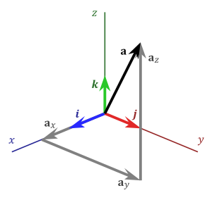
In order to calculate with vectors, the graphical representation may be too cumbersome. Vectors in an n-dimensional Euclidean space can be represented in a Cartesian coordinate system. The endpoint of a vector can be identified with an ordered list of n real numbers (n-tuple). These numbers are the coordinates of the endpoint of the vector, with respect to a given Cartesian coordinate system, and are typically called the scalar components (or scalar projections) of the vector on the axes of the coordinate system.

As an example in two dimensions (see figure), the vector from the origin O = (0,0) to the point A = (2,3) is simply written as

$\mathbf{a} = (2,3).$

The notion that the tail of the vector coincides with the origin is implicit and easily understood. Thus, the more explicit notation $\overrightarrow{OA}$ is usually not deemed necessary and very rarely used.

In three dimensional Euclidean space (or $\mathbb{R}^3$), vectors are identified with triples of scalar components:

$\mathbf{a} = (a_1, a_2, a_3).$

also written

$\mathbf{a} = (a_x, a_y, a_z).$

These numbers are often arranged into a column vector or row vector, particularly when dealing with matrices, as follows:

$\mathbf{a} = \begin{bmatrix} a_1\\ a_2\\ a_3\\ \end{bmatrix}$

$\mathbf{a} = [ a_1\ a_2\ a_3 ].$

Another way to represent a vector in n-dimensions is to introduce the standard basis vectors. For instance, in three dimensions, there are three of them:

${\mathbf e}_1 = (1,0,0),\ {\mathbf e}_2 = (0,1,0),\ {\mathbf e}_3 = (0,0,1).$

These have the intuitive interpretation as vectors of unit length pointing up the x, y, and z axis of a Cartesian coordinate system, respectively, and they are sometimes referred to as versors of those axes. In terms of these, any vector a in $\mathbb{R}^3$ can be expressed in the form:

$\mathbf{a} = (a_1,a_2,a_3) = a_1(1,0,0) + a_2(0,1,0) + a_3(0,0,1), \$

or

$\mathbf{a} = \mathbf{a}_1 + \mathbf{a}_2 + \mathbf{a}_3 = a_1{\mathbf e}_1 + a_2{\mathbf e}_2 + a_3{\mathbf e}_3,$

where a₁, a₂, a₃ are called the vector components (or vector projections) of a on the basis vectors or, equivalently, on the corresponding Cartesian axes x, y, and z (see figure), while a₁, a₂, a₃ are the respective scalar components (or scalar projections).

In introductory physics textbooks, the standard basis vectors are often instead denoted $\mathbf{i},\mathbf{j},\mathbf{k}$ (or $\mathbf{\hat{x}}, \mathbf{\hat{y}}, \mathbf{\hat{z}}$, in which the hat symbol ^ typically denotes unit vectors). In this case, the scalar and vector components are denoted a_x, a_y, a_z, and a_x, a_y, a_z. Thus,

$\mathbf{a} = \mathbf{a}_x + \mathbf{a}_y + \mathbf{a}_z = a_x{\mathbf i} + a_y{\mathbf j} + a_z{\mathbf k}.$

The notation e_i is compatible with the index notation and the summation convention commonly used in higher level mathematics, physics, and engineering.

Decomposition

As explained above a vector is often described by a set of vector components that are mutually perpendicular and add up to form the given vector. Typically, these components are the projections of the vector on a set of reference axes (or basis vectors). The vector is said to be decomposed or resolved with respect to that set.

Illustration of tangential and normal components of a vector to a surface.

However, the decomposition of a vector into components is not unique, because it depends on the choice of the axes on which the vector is projected.

Moreover, the use of Cartesian versors such as $\mathbf{\hat{x}}, \mathbf{\hat{y}}, \mathbf{\hat{z}}$ as a basis in which to represent a vector is not mandated. Vectors can also be expressed in terms of the versors of a Cylindrical coordinate system ($\boldsymbol{\hat{\rho}}, \boldsymbol{\hat{\phi}}, \mathbf{\hat{z}}$) or Spherical coordinate system ($\mathbf{\hat{r}}, \boldsymbol{\hat{\theta}}, \boldsymbol{\hat{\phi}}$). The latter two choices are more convenient for solving problems which possess cylindrical or spherical symmetry respectively.

The choice of a coordinate system doesn't affect the properties of a vector or its behaviour under transformations.

A vector can be also decomposed with respect to "non-fixed" axes which change their orientation as a function of time or space. For example, a vector in three dimensional space can be decomposed with respect to two axes, respectively normal, and tangent to a surface (see figure). Moreover, the radial and tangential components of a vector relate to the radius of rotation of an object. The former is parallel to the radius and the latter is orthogonal to it.^[8]

In these cases, each of the components may be in turn decomposed with respect to a fixed coordinate system or basis set (e.g., a global coordinate system, or inertial reference frame).

Basic properties

The following section uses the Cartesian coordinate system with basis vectors

${\mathbf e}_1 = (1,0,0),\ {\mathbf e}_2 = (0,1,0),\ {\mathbf e}_3 = (0,0,1)$

and assume that all vectors have the origin as a common base point. A vector a will be written as

${\mathbf a} = a_1{\mathbf e}_1 + a_2{\mathbf e}_2 + a_3{\mathbf e}_3.$

Equality

Two vectors are said to be equal if they have the same magnitude and direction. Equivalently they will be equal if their coordinates are equal. So two vectors

${\mathbf a} = a_1{\mathbf e}_1 + a_2{\mathbf e}_2 + a_3{\mathbf e}_3$

and

${\mathbf b} = b_1{\mathbf e}_1 + b_2{\mathbf e}_2 + b_3{\mathbf e}_3$

are equal if

$a_1 = b_1,\quad a_2=b_2,\quad a_3=b_3.\,$

Addition and subtraction

Assume now that a and b are not necessarily equal vectors, but that they may have different magnitudes and directions. The sum of a and b is

$\mathbf{a}+\mathbf{b} =(a_1+b_1)\mathbf{e_1} +(a_2+b_2)\mathbf{e_2} +(a_3+b_3)\mathbf{e_3}.$

The addition may be represented graphically by placing the start of the arrow b at the tip of the arrow a, and then drawing an arrow from the start of a to the tip of b. The new arrow drawn represents the vector a + b, as illustrated below:

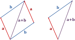
This addition method is sometimes called the parallelogram rule because a and b form the sides of a parallelogram and a + b is one of the diagonals. If a and b are bound vectors that have the same base point, it will also be the base point of a + b. One can check geometrically that a + b = b + a and (a + b) + c = a + (b + c).

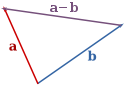
The difference of a and b is

$\mathbf{a}-\mathbf{b} =(a_1-b_1)\mathbf{e_1} +(a_2-b_2)\mathbf{e_2} +(a_3-b_3)\mathbf{e_3}.$

Subtraction of two vectors can be geometrically defined as follows: to subtract b from a, place the end points of a and b at the same point, and then draw an arrow from the tip of b to the tip of a. That arrow represents the vector a − b, as illustrated below:

Scalar multiplication

Scalar multiplication of a vector by a factor of 3 stretches the vector out.

The scalar multiplications 2a and −a of a vector a

A vector may also be multiplied, or re-scaled, by a real number r. In the context of conventional vector algebra, these real numbers are often called scalars (from scale) to distinguish them from vectors. The operation of multiplying a vector by a scalar is called scalar multiplication. The resulting vector is

$r\mathbf{a}=(ra_1)\mathbf{e_1} +(ra_2)\mathbf{e_2} +(ra_3)\mathbf{e_3}.$

Intuitively, multiplying by a scalar r stretches a vector out by a factor of r. Geometrically, this can be visualized (at least in the case when r is an integer) as placing r copies of the vector in a line where the endpoint of one vector is the initial point of the next vector.

If r is negative, then the vector changes direction: it flips around by an angle of 180°. Two examples (r = −1 and r = 2) are given below:

Scalar multiplication is distributive over vector addition in the following sense: r(a + b) = ra + rb for all vectors a and b and all scalars r. One can also show that a − b = a + (−1)b.

Length

The length or magnitude or norm of the vector a is denoted by ||a|| or, less commonly, |a|, which is not to be confused with the absolute value (a scalar "norm").

The length of the vector a can be computed with the Euclidean norm

$\left\|\mathbf{a}\right\|=\sqrt{{a_1}^2+{a_2}^2+{a_3}^2}$

which is a consequence of the Pythagorean theorem since the basis vectors e₁, e₂, e₃ are orthogonal unit vectors.

This happens to be equal to the square root of the dot product, discussed below, of the vector with itself:

$\left\|\mathbf{a}\right\|=\sqrt{\mathbf{a}\cdot\mathbf{a}}.$

Unit vector

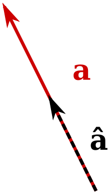The normalization of a vector a into a unit vector â

Main article: Unit vector

A unit vector is any vector with a length of one; normally unit vectors are used simply to indicate direction. A vector of arbitrary length can be divided by its length to create a unit vector. This is known as normalizing a vector. A unit vector is often indicated with a hat as in â.

To normalize a vector a = [a₁, a₂, a₃], scale the vector by the reciprocal of its length ||a||. That is:

$\mathbf{\hat{a}} = \frac{\mathbf{a}}{\left\|\mathbf{a}\right\|} = \frac{a_1}{\left\|\mathbf{a}\right\|}\mathbf{e_1} + \frac{a_2}{\left\|\mathbf{a}\right\|}\mathbf{e_2} + \frac{a_3}{\left\|\mathbf{a}\right\|}\mathbf{e_3}$

Null vector

Main article: Null vector

The null vector (or zero vector) is the vector with length zero. Written out in coordinates, the vector is (0,0,0), and it is commonly denoted $\vec{0}$, or 0, or simply 0. Unlike any other vector it has an arbitrary or indeterminate direction, and cannot be normalized (that is, there is no unit vector which is a multiple of the null vector). The sum of the null vector with any vector a is a (that is, 0+a=a).

Dot product

Main article: dot product

The dot product of two vectors a and b (sometimes called the inner product, or, since its result is a scalar, the scalar product) is denoted by a ∙ b and is defined as:

$\mathbf{a}\cdot\mathbf{b} =\left\|\mathbf{a}\right\|\left\|\mathbf{b}\right\|\cos\theta$

where θ is the measure of the angle between a and b (see trigonometric function for an explanation of cosine). Geometrically, this means that a and b are drawn with a common start point and then the length of a is multiplied with the length of that component of b that points in the same direction as a.

The dot product can also be defined as the sum of the products of the components of each vector as

$\mathbf{a} \cdot \mathbf{b} = a_1 b_1 + a_2 b_2 + a_3 b_3.$

Cross product

Main article: Cross product

The cross product (also called the vector product or outer product) is only meaningful in three or seven dimensions. The cross product differs from the dot product primarily in that the result of the cross product of two vectors is a vector. The cross product, denoted a × b, is a vector perpendicular to both a and b and is defined as

$\mathbf{a}\times\mathbf{b} =\left\|\mathbf{a}\right\|\left\|\mathbf{b}\right\|\sin(\theta)\,\mathbf{n}$

where θ is the measure of the angle between a and b, and n is a unit vector perpendicular to both a and b which completes a right-handed system. The right-handedness constraint is necessary because there exist two unit vectors that are perpendicular to both a and b, namely, n and (–n).

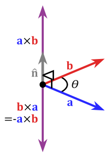An illustration of the cross product

The cross product a × b is defined so that a, b, and a × b also becomes a right-handed system (but note that a and b are not necessarily orthogonal). This is the right-hand rule.

The length of a × b can be interpreted as the area of the parallelogram having a and b as sides.

The cross product can be written as

${\mathbf a}\times{\mathbf b} = (a_2 b_3 - a_3 b_2) {\mathbf e}_1 + (a_3 b_1 - a_1 b_3) {\mathbf e}_2 + (a_1 b_2 - a_2 b_1) {\mathbf e}_3.$

For arbitrary choices of spatial orientation (that is, allowing for left-handed as well as right-handed coordinate systems) the cross product of two vectors is a pseudovector instead of a vector (see below).

Scalar triple product

Main article: Scalar triple product

The scalar triple product (also called the box product or mixed triple product) is not really a new operator, but a way of applying the other two multiplication operators to three vectors. The scalar triple product is sometimes denoted by (a b c) and defined as:

$(\mathbf{a}\ \mathbf{b}\ \mathbf{c}) =\mathbf{a}\cdot(\mathbf{b}\times\mathbf{c}).$

It has three primary uses. First, the absolute value of the box product is the volume of the parallelepiped which has edges that are defined by the three vectors. Second, the scalar triple product is zero if and only if the three vectors are linearly dependent, which can be easily proved by considering that in order for the three vectors to not make a volume, they must all lie in the same plane. Third, the box product is positive if and only if the three vectors a, b and c are right-handed.

In components (with respect to a right-handed orthonormal basis), if the three vectors are thought of as rows (or columns, but in the same order), the scalar triple product is simply the determinant of the 3-by-3 matrix having the three vectors as rows

$(\mathbf{a}\ \mathbf{b}\ \mathbf{c})=\left|\begin{pmatrix} a_1 & a_2 & a_3 \\ b_1 & b_2 & b_3 \\ c_1 & c_2 & c_3 \\ \end{pmatrix}\right|.$

The scalar triple product is linear in all three entries and anti-symmetric in the following sense:

$(\mathbf{a}\ \mathbf{b}\ \mathbf{c}) = (\mathbf{c}\ \mathbf{a}\ \mathbf{b}) = (\mathbf{b}\ \mathbf{c}\ \mathbf{a})= -(\mathbf{a}\ \mathbf{c}\ \mathbf{b}) = -(\mathbf{b}\ \mathbf{a}\ \mathbf{c}) = -(\mathbf{c}\ \mathbf{b}\ \mathbf{a}).$

Multiple Cartesian bases

All examples thus far have dealt with vectors expressed in terms of the same basis, namely, e₁,e₂,e₃. However, a vector can be expressed in terms of any number of different bases that are not necessarily aligned with each other, and still remain the same vector. For example, using the vector a from above,

$\mathbf{a} = a_1\mathbf{e}_1 + a_2\mathbf{e}_2 + a_3\mathbf{e}_3 = u\mathbf{n}_1 + v\mathbf{n}_2 + w\mathbf{n}_3$

where n₁,n₂,n₃ form another orthonormal basis not aligned with e₁,e₂,e₃. The values of u, v, and w are such that the resulting vector sum is exactly a.

It is not uncommon to encounter vectors known in terms of different bases (for example, one basis fixed to the Earth and a second basis fixed to a moving vehicle). In order to perform many of the operations defined above, it is necessary to know the vectors in terms of the same basis. One simple way to express a vector known in one basis in terms of another uses column matrices that represent the vector in each basis along with a third matrix containing the information that relates the two bases. For example, in order to find the values of u, v, and w that define a in the n₁,n₂,n₃ basis, a matrix multiplication may be employed in the form

$\begin{bmatrix} u \\ v \\ w \\ \end{bmatrix} = \begin{bmatrix} c_{11} & c_{12} & c_{13} \\ c_{21} & c_{22} & c_{23} \\ c_{31} & c_{32} & c_{33} \end{bmatrix} \begin{bmatrix} a_1 \\ a_2 \\ a_3 \end{bmatrix}$

where each matrix element c_jk is the direction cosine relating n_j to e_k.^[9] The term direction cosine refers to the cosine of the angle between two unit vectors, which is also equal to their dot product.^[9]

By referring collectively to e₁,e₂,e₃ as the e basis and to n₁,n₂,n₃ as the n basis, the matrix containing all the c_jk is known as the "transformation matrix from e to n", or the "rotation matrix from e to n" (because it can be imagined as the "rotation" of a vector from one basis to another), or the "direction cosine matrix from e to n"^[9] (because it contains direction cosines).

The properties of a rotation matrix are such that its inverse is equal to its transpose. This means that the "rotation matrix from e to n" is the transpose of "rotation matrix from n to e".

By applying several matrix multiplications in succession, any vector can be expressed in any basis so long as the set of direction cosines is known relating the successive bases.^[9]

Other dimensions

With the exception of the cross and triple products, the above formula generalise to two dimensions and higher dimensions. For example, addition generalises to two dimensions the addition of

$(a_1{\mathbf e}_1 + a_2{\mathbf e}_2)+(b_1{\mathbf e}_1 + b_2{\mathbf e}_2) = (a_1+b_1){\mathbf e}_1 + (a_2+b_2){\mathbf e}_2$

and in four dimension

$\begin{align}(a_1{\mathbf e}_1 + a_2{\mathbf e}_2 + a_3{\mathbf e}_3 + a_4{\mathbf e}_4) &+ (b_1{\mathbf e}_1 + b_2{\mathbf e}_2 + b_3{\mathbf e}_3 + b_4{\mathbf e}_4) =\\ (a_1+b_1){\mathbf e}_1 + (a_2+b_2){\mathbf e}_2 &+ (a_3+b_3){\mathbf e}_3 + (a_4+b_4){\mathbf e}_4.\end{align}$

The cross product generalises to the exterior product, whose result is a bivector, which in general is not a vector. In two dimensions this is simply a scalar

$(a_1{\mathbf e}_1 + a_2{\mathbf e}_2)\wedge(b_1{\mathbf e}_1 + b_2{\mathbf e}_2) = a_1 b_2 - a_2 b_1.$

The seven-dimensional cross product is similar to the cross product in that its result is a seven-dimensional vector orthogonal to the two arguments.

Physics

Vectors have many uses in physics and other sciences.

Length and units

In abstract vector spaces, the length of the arrow depends on a dimensionless scale. If it represents, for example, a force, the "scale" is of physical dimension length/force. Thus there is typically consistency in scale among quantities of the same dimension, but otherwise scale ratios may vary; for example, if "1 newton" and "5 m" are both represented with an arrow of 2 cm, the scales are 1:250 and 1 m:50 N respectively. Equal length of vectors of different dimension has no particular significance unless there is some proportionality constant inherent in the system that the diagram represents. Also length of a unit vector (of dimension length, not length/force, etc.) has no coordinate-system-invariant significance.

Vector-valued functions

Main article: Vector-valued function

Often in areas of physics and mathematics, a vector evolves in time, meaning that it depends on a time parameter t. For instance, if r represents the position vector of a particle, then r(t) gives a parametric representation of the trajectory of the particle. Vector-valued functions can be differentiated and integrated by differentiating or integrating the components of the vector, and many of the familiar rules from calculus continue to hold for the derivative and integral of vector-valued functions.

Position, velocity and acceleration

The position of a point x=(x₁, x₂, x₃) in three dimensional space can be represented as a position vector whose base point is the origin

${\mathbf x} = x_1 {\mathbf e}_1 + x_2{\mathbf e}_2 + x_3{\mathbf e}_3.$

The position vectors has dimensions of length.

Given two points x=(x₁, x₂, x₃), y=(y₁, y₂, y₃) their displacement is a vector

${\mathbf y}-{\mathbf x}=(y_1-x_1){\mathbf e}_1 + (y_2-x_2){\mathbf e}_2 + (y_3-x_3){\mathbf e}_3.$

which specifies the position of y relative to x. The length of this vector gives the straight line distance from x to y. Displacement has the dimensions of length.

The velocity v of a point or particle is a vector, its length gives the speed. For constant velocity the position at time t will be

${\mathbf x}_t= t {\mathbf v} + {\mathbf x}_0,$

where x₀ is the position at time t=0. Velocity is the time derivative of position. Its dimensions are length/time.

Acceleration a of a point is vector which is the time derivative of velocity. Its dimensions are length/time².

Force, energy, work

Force is a vector with dimensions of mass×length/time² and Newton's second law is the scalar multiplication

${\mathbf F} = m{\mathbf a}$

Work is the dot product of force and displacement

$E = {\mathbf F} \cdot ({\mathbf x}_2 - {\mathbf x}_1).$

Vectors as directional derivatives

A vector may also be defined as a directional derivative: consider a function f(x^α) and a curve x^α(τ). Then the directional derivative of f is a scalar defined as

$\frac{df}{d\tau} = \sum_{\alpha=1}^n \frac{dx^\alpha}{d\tau}\frac{\partial f}{\partial x^\alpha}.$

where the index α is summed over the appropriate number of dimensions (for example, from 1 to 3 in 3-dimensional Euclidean space, from 0 to 3 in 4-dimensional spacetime, etc.). Then consider a vector tangent to x^α(τ):

$t^\alpha = \frac{dx^\alpha}{d\tau}.$

The directional derivative can be rewritten in differential form (without a given function f) as

$\frac{d}{d\tau} = \sum_\alpha t^\alpha\frac{\partial}{\partial x^\alpha}.$

Therefore any directional derivative can be identified with a corresponding vector, and any vector can be identified with a corresponding directional derivative. A vector can therefore be defined precisely as

$\mathbf{a} \equiv a^\alpha \frac{\partial}{\partial x^\alpha}.$

Vectors, pseudovectors, and transformations

An alternative characterization of Euclidean vectors, especially in physics, describes them as lists of quantities which behave in a certain way under a coordinate transformation. A contravariant vector is required to have components that "transform like the coordinates" under changes of coordinates such as rotation and dilation. The vector itself does not change under these operations; instead, the components of the vector make a change that cancels the change in the spatial axes, in the same way that co-ordinates change. In other words, if the reference axes were rotated in one direction, the component representation of the vector would rotate in exactly the opposite way. Similarly, if the reference axes were stretched in one direction, the components of the vector, like the co-ordinates, would reduce in an exactly compensating way. Mathematically, if the coordinate system undergoes a transformation described by an invertible matrix M, so that a coordinate vector x is transformed to x′ = Mx, then a contravariant vector v must be similarly transformed via v′ = Mv. This important requirement is what distinguishes a contravariant vector from any other triple of physically meaningful quantities. For example, if v consists of the x, y, and z-components of velocity, then v is a contravariant vector: if the coordinates of space are stretched, rotated, or twisted, then the components of the velocity transform in the same way. On the other hand, for instance, a triple consisting of the length, width, and height of a rectangular box could make up the three components of an abstract vector, but this vector would not be contravariant, since rotating the box does not change the box's length, width, and height. Examples of contravariant vectors include displacement, velocity, electric field, momentum, force, and acceleration.

In the language of differential geometry, the requirement that the components of a vector transform according to the same matrix of the coordinate transition is equivalent to defining a contravariant vector to be a tensor of contravariant rank one. Alternatively, a contravariant vector is defined to be a tangent vector, and the rules for transforming a contravariant vector follow from the chain rule.

Some vectors transform like contravariant vectors, except that when they are reflected through a mirror, they flip and gain a minus sign. A transformation that switches right-handedness to left-handedness and vice versa like a mirror does is said to change the orientation of space. A vector which gains a minus sign when the orientation of space changes is called a pseudovector or an axial vector. Ordinary vectors are sometimes called true vectors or polar vectors to distinguish them from pseudovectors. Pseudovectors occur most frequently as the cross product of two ordinary vectors.

One example of a pseudovector is angular velocity. Driving in a car, and looking forward, each of the wheels has an angular velocity vector pointing to the left. If the world is reflected in a mirror which switches the left and right side of the car, the reflection of this angular velocity vector points to the right, but the actual angular velocity vector of the wheel still points to the left, corresponding to the minus sign. Other examples of pseudovectors include magnetic field, torque, or more generally any cross product of two (true) vectors.

This distinction between vectors and pseudovectors is often ignored, but it becomes important in studying symmetry properties. See parity (physics).

See also

• Affine space, which distinguishes between vectors and points
• Four-vector, a non-Euclidean vector in Minkowski space (i.e. four-dimensional spacetime), important in relativity
• Normal vector
• Null vector
• Pseudovector
• Tangential and normal components (of a vector)
• Unit vector
• Vector calculus
• Vector-valued function
• Vector bundle
• Vector notation
• Function space
• Banach space
• Hilbert space
• Coordinate system
• Complex number
• Quaternion
• Grassmann's Ausdehnungslehre
• Clifford algebra
• Tensor
• Covariance and contravariance of vectors

Notes

1. ^ Ivanov 2001
2. ^ Heinbockel 2001
3. ^ Ito 1993, p. 1678; Pedoe 1988
4. ^ Latin: vectus, perfect participle of vehere, "to carry"/ veho = "I carry". For historical development of the word vector, see "vector n.". Oxford English Dictionary. Oxford University Press. 2nd ed. 1989. and Jeff Miller. "Earliest Known Uses of Some of the Words of Mathematics". http://jeff560.tripod.com/v.html. Retrieved 2007-05-25. .
5. ^ Ito 1993, p. 1678
6. ^ Thermodynamics and Differential Forms
7. ^ ^{a b} Michael J. Crowe, A History of Vector Analysis; see also his lecture notes on the subject.
8. ^ U. Guelph Physics Dept., "TORQUE AND ANGULAR ACCELERATION"
9. ^ ^{a b c d} Kane & Levinson 1996, pp. 20–22

References

Mathematical treatments

• Apostol, T. (1967). Calculus, Vol. 1: One-Variable Calculus with an Introduction to Linear Algebra. John Wiley and Sons. ISBN 978-0471000051. 
• Apostol, T. (1969). Calculus, Vol. 2: Multi-Variable Calculus and Linear Algebra with Applications. John Wiley and Sons. ISBN 978-0471000075. 
• Kane, Thomas R.; Levinson, David A. (1996), Dynamics Online, Sunnyvale, California: OnLine Dynamics, Inc. 
• Heinbockel, J. H. (2001), Introduction to Tensor Calculus and Continuum Mechanics, Trafford Publishing, ISBN 1553691334, http://www.math.odu.edu/~jhh/counter2.html 
• Ito, Kiyosi (1993), Encyclopedic Dictionary of Mathematics (2nd ed.), MIT Press, ISBN 978-0-262-59020-4 
• Ivanov, A.B. (2001), "Vector, geometric", in Hazewinkel, Michiel, Encyclopaedia of Mathematics, Springer, ISBN 978-1556080104, http://eom.springer.de/V/v096340.htm 
• Pedoe, D. (1988). Geometry: A comprehensive course. Dover. ISBN 0-486-65812-0. .

Physical treatments

• Aris, R. (1990). Vectors, Tensors and the Basic Equations of Fluid Mechanics. Dover. ISBN 978-0486661100. 
• Feynman, R., Leighton, R., and Sands, M. (2005). "Chapter 11". The Feynman Lectures on Physics, Volume I (2nd ed ed.). Addison Wesley. ISBN 978-0805390469. 

External links

• Online vector identities (PDF)
• Introducing Vectors A conceptual introduction (applied mathematics)
• Addition of forces (vectors) Java Applet
• French tutorials on vectors and their application to video games