- Constraint satisfaction dual problem
-
The dual problem is a reformulation of a constraint satisfaction problem expressing each constraint of the original problem as a variable. Dual problems only contain binary constraints, and are therefore solvable by algorithms tailored for such problems. The join graphs and join trees of a constraint satisfaction problem are graphs representing its dual problem or a problem obtained from the dual problem removing some redundant constraints.
Contents
The dual problem
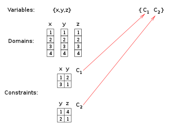
The dual problem of a constraint satisfaction problem contains a variable for each constraint of the original problem. Its domains and constraints are built so to enforce a sort of equivalence to the original problem. In particular, the domain of a variable of the dual problem contains one element for each tuple satisfying the corresponding original constraint. This way, a dual variable can take a value if and only if the corresponding original constraint is satisfied by the corresponding tuple.
The constraints of the dual problem forbid two dual variables to take values that correspond to two incompatible tuples. Without these constraints, one dual variable may take the value corresponding to the tuple x = 1,y = 2 while another dual variable takes the value corresponding to y = 3,z = 1, which assigns a different value to y.
More generally, the constraints of the dual problem enforce the same values for all variables shared by two constraints. If two dual variables correspond to constraints sharing some variables, the dual problem contains a constraint between them, enforcing equality of all shared variables.
The dual variables are the constraints of the original problem. 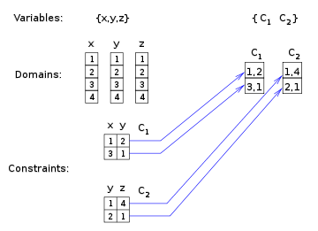
The domain of each dual variable is the set of tuples of the corresponding original constraint. 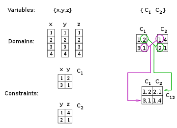
The dual constraints enforce the dual variables (original constraints) to have values (original tuples) that contain equal values of the original variables. In this example, the original constraints C1 and C2 share the variable y. In the dual problem, the variables C1 and C2 are allowed to have values (1,2) and (2,1) because these values agree on y = 2.
In the dual problem, all constraints are binary. They all enforce two values, which are tuples, to agree on one or more original variables.
The dual graph is a representation of how variables are constrained in the dual problem. More precisely, the dual graph contains a node for each dual variable and an edge for every constraint between them. In addition, the edge between two variables is labeled by the original variables that are enforced equal between these two dual variables.
The dual graph can be built directly from the original problem: it contains a vertex for each constraint, and an edge between every two constraints sharing variables; such an edge is labeled by these shared variables.
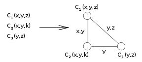
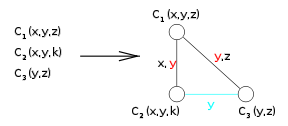
A dual graph. An edge between two constraints corresponds to a dual constraint enforcing equality of their shared variables. For example, the edge labeled x,y between C1 and C2 indicates that the dual problem contains a constraint between C1 and C2, and this constraint enforces values (tuples) that match on x and y. Join graphs and join trees
In the dual graph, some constraints may be unnecessary. Indeed, dual constraints enforces equality of original variables, and some constraints may be redundant because of transitivity of equality. For example, if C2 and C1 are joined by an edge whose label contains y, and so are C1 and C3, equality of y in all three dual variables is guaranteed. As a result, a dual constraint between C2 and C3 enforcing equality of y is not necessary, and could be removed if present.
Since equality of y is enforced by other dual constraints, the one between C2 and C3 can be dropped. A graph obtained from the dual graph by removing some redundant edges is called a join graph. If it is a tree, it is called a join tree. The dual problem can be solved from a join graph since all removed edges are redundant. In turn, the problem can be solved efficiently if that join graph is a tree, using algorithms tailored for acyclic constraint satisfaction problems.
Finding a join tree, if any, can be done exploiting the following property: if a dual graph has a join tree, then the maximal-weight spanning trees of the graph are all join trees, if edges are weighted by the number of variables the corresponding constraints enforce to be equal. An algorithm for finding a join tree, if any, proceeds as follows. In the first step, edges are assigned weights: if two nodes represent constraints that share n variables, the edge joining them is assigned weight n. In the second step, a maximal-weight spanning tree is searched for. Once one is found, it is checked whether it enforces the required equality of variables. If this is the case, this spanning tree is a join tree.
Another method for finding out whether a constraint satisfaction problem has a join tree uses the primal graph of the problem, rather than the dual graph. The primal graph of a constraint satisfaction problem is a graph whose nodes are problem variables and whose edges represent the presence of two variables in the same constraint. A join tree for the problem exists if:
- the primal graph is chordal;
- the variables of every maximal clique of the primal graph are the scope of a constraint and vice versa; this property is called conformality.
In turn, chordality can be checked using a max-cardinality ordering of the variables. Such an ordering can also be used, if the two conditions above are met, for finding a join tree of the problem. Ordering constraints by their highest variable according to the ordering, an algorithm for producing a join tree proceeds from the last to the first constraint; at each step, a constraint is connected to the constraint that shares a maximal number of variables with it among the constraints that precede it in the ordering.
Extensions
Not all constraint satisfaction problems have a join tree. However, problems can be modified to acquire a join tree. Join-tree clustering is a specific method to modify problems in such a way they acquire a joint tree. This is done by merging constraints, which typically increases the size of the problem; however, solving the resulting problem is easy, as it is for all problems that have a join tree.
Decomposition methods generalize join-tree clustering by grouping variables in such a way the resulting problem has a join tree. Decomposition methods directly associate a tree with problems; the nodes of this tree are associated varibables and/or constraints of the original problem. By merging constraints based on this tree, one can produce a problem that has a join tree, and this join tree can be easily derived from the decomposition tree. Alternatively, one can build a binary acyclic problem directly from the decomposition tree.
References
- Dechter, Rina (2003). Constraint Processing. Morgan Kaufmann. http://www.ics.uci.edu/~dechter/books/index.html. ISBN 978-1-55860-890-0
- Downey, Rod; M. Fellows (1997). Parameterized complexity. Springer. http://www.springer.com/sgw/cda/frontpage/0,11855,5-0-22-1519914-0,00.html?referer=www.springer.de%2Fcgi-bin%2Fsearch_book.pl%3Fisbn%3D0-387-94883-X. ISBN 978-0-387-94883-6
- Georg Gottlob, Nicola Leone, Francesco Scarcello (2001). "Hypertree Decompositions: A Survey". MFCS 2001. pp. 37–57. http://www.springerlink.com/(rqc54x55rqwetq55eco03ymp)/app/home/contribution.asp?referrer=parent&backto=issue,5,61;journal,1765,3346;linkingpublicationresults,1:105633,1.
See also
Categories:


Wikimedia Foundation. 2010.