- Möbius transformation
-
Not to be confused with Möbius transform or Möbius function.
In geometry, a Möbius transformation of the plane is a rational function of the form
of one complex variable z; here the coefficients a, b, c, d are complex numbers satisfying ad − bc ≠ 0.
Möbius transformations are named in honor of August Ferdinand Möbius, although they are also called homographic transformations, linear fractional transformations, or fractional linear transformations.
Overview
Möbius transformations are defined on the extended complex plane (i.e. the complex plane augmented by the point at infinity):
This extended complex plane can be thought of as a sphere, the Riemann sphere, or as the complex projective line. Every Möbius transformation is a bijective conformal map of the Riemann sphere to itself. Indeed, every such map is by necessity a Möbius transformation.
The set of all Möbius transformations forms a group under composition called the Möbius group. It is the automorphism group of the Riemann sphere (when considered as a Riemann surface) and is sometimes denoted
 .
.
The Möbius group is isomorphic to the group of orientation-preserving isometries of hyperbolic 3-space and therefore plays an important role when studying hyperbolic 3-manifolds.
In physics, the identity component of the Lorentz group acts on the celestial sphere in the same way that the Möbius group acts on the Riemann sphere. In fact, these two groups are isomorphic. An observer who accelerates to relativistic velocities will see the pattern of constellations as seen near the Earth continuously transform according to infinitesimal Möbius transformations. This observation is often taken as the starting point of twistor theory.
Certain subgroups of the Möbius group form the automorphism groups of the other simply-connected Riemann surfaces (the complex plane and the hyperbolic plane). As such, Möbius transformations play an important role in the theory of Riemann surfaces. The fundamental group of every Riemann surface is a discrete subgroup of the Möbius group (see Fuchsian group and Kleinian group). A particularly important discrete subgroup of the Möbius group is the modular group; it is central to the theory of many fractals, modular forms, elliptic curves and Pellian equations.
Möbius transformations can be more generally defined in spaces of dimension n>2 as the bijective conformal orientation-preserving maps from the n-sphere to the n-sphere. Such a transformation is the most general form of conformal mapping of a domain. According to Liouville's theorem a Möbius transformation can be expressed as a composition of translations, similarities, orthogonal transformations and inversions.
Definition
The general form of a Möbius transformation is given by
where a, b, c, d are any complex numbers satisfying ad − bc ≠ 0. (If ad = bc the rational function defined above is a constant and is not considered a Möbius transformation.) In case c≠0 this definition is extended to the whole Riemann sphere by defining
if c=0 we define
This turns f(z) into a bijective holomorphic function from the Riemann sphere to the Riemann sphere.
The set of all Möbius transformations forms a group under composition. This group can be given the structure of a complex manifold in such a way that composition and inversion are holomorphic maps. The Möbius group is then a complex Lie group. The Möbius group is usually denoted
 as it is the automorphism group of the Riemann sphere.
Decomposition and elementary properties
A Möbius transformation is equivalent to a sequence of simpler transformations. Let:
 (translation by d/c)
 (inversion and reflection with respect to the real axis)
 (dilation and rotation)
 (translation by a/c)
then these functions can be composed, giving
This decomposition makes many properties of the Möbius transformation obvious.
The existence of the inverse Möbius transformation and its explicit formula are easily derived by the composition of the inverse functions of the simpler transformations. That is, define functions g1,g2,g3,g4 such that each gi is the inverse of fi. Then the composition
gives a formula for the inverse.
Preservation of angles and generalized circles
From this decomposition, we see that Möbius transformations carry over all non-trivial properties of circle inversion. For example, the preservation of angles is reduced to proving that circle inversion preserves angles since the other types of transformations are dilation and isometries (translation, reflection, rotation), which trivially preserve angles.
Furthermore, Möbius transformations map generalized circles to generalized circles since circle inversion has this property. A generalized circle is either a circle or a line, the latter being considered as a circle through the point at infinity. Note that a Möbius transformation does not necessarily map circles to circles and lines to lines: it can mix the two. Even if it maps a circle to another circle, it does not necessarily map the first circle's center to the second circle's center.
Cross-ratio preservation
Cross-ratios are invariant under Möbius transformations. That is, if a Möbius transformation maps four distinct points z1,z2,z3,z4 to four distinct points w1,w2,w3,w4 respectively, then
If one of the points z1,z2,z3,z4 is the point at infinity, then the cross-ratio has to be defined by taking the appropriate limit; e.g. the cross-ratio of
 is
isProjective matrix representations
With every invertible complex 2-by-2 matrix
we can associate the Möbius transformation
The condition ad − bc ≠ 0 is equivalent to the condition that the determinant of above matrix be nonzero, i.e. that the matrix be invertible.
It is straightforward to check that then the product of two matrices will be associated with the composition of the two corresponding Möbius transformations. In other words, the map
from the general linear group GL(2,C) to the Möbius group, which sends the matrix
 to the transformation f, is a group homomorphism.
Note that any matrix obtained by multiplying
 by a complex scalar λ determines the same transformation, so a Möbius transformation determines its matrix only up to scalar multiples. In other words: the kernel of π consists of all scalar multiples of the identity matrix I, and the first isomorphism theorem of group theory states that the quotient group GL(2,C)/(CI) is isomorphic to the Möbius group. This quotient group is known as the projective linear group and is usually denoted PGL(2,C).
The same identification of PGL(2,K) with the group of fractional linear transformations and with the group of projective linear automorphisms of the projective line holds over any field K, a fact of algebraic interest, particularly for finite fields, though the case of the complex numbers has the greatest geometric interest.
The natural action of PGL(2,C) on the complex projective line CP1 is exactly the natural action of the Möbius group on the Riemann sphere, where the projective line CP1 and the Riemann sphere are identified as follows:
Here [z1:z2] are homogeneous coordinates on CP1; the point [1:0] corresponds to the point ∞ of the Riemann sphere. By using homogeneous coordinates, many concrete calculations involving Möbius transformations can be simplified, since no case distinctions dealing with ∞ are required.
If one restricts
to matrices of determinant one, the map π restricts to a surjective map from the special linear group SL(2,C) to the Möbius group; in the restricted setting the kernel is formed by plus and minus the identity, and the quotient group SL(2,C)/{±I}, denoted by PSL(2,C), is therefore also isomorphic to the Möbius group:From this we see that the Möbius group is a 3-dimensional complex Lie group (or a 6-dimensional real Lie group). It is a semisimple non-compact Lie group.
Note that there are precisely two matrices with unit determinant which can be used to represent any given Möbius transformation. That is, SL(2,C) is a double cover of PSL(2,C). Since SL(2,C) is simply-connected it is the universal cover of the Möbius group. Therefore the fundamental group of the Möbius group is Z2.
Specifying a transformation by three points
Given a set of three distinct points z1, z2, z3 on the Riemann sphere and a second set of distinct points w1, w2, w3, there exists precisely one Möbius transformation f(z) which maps the zs to the ws, i.e. with f(zi) = wi for i=1,2,3. (In other words: the action of the Möbius group on the Riemann sphere is sharply 3-transitive.) There are several ways to determine f(z) from the given sets of points.
Mapping first to 0, 1, ∞
It is easy to check that the Möbius transformation
with matrix
maps z1, z2, z3 to 0, 1, ∞, respectively. (If one of the zi is ∞, then the proper formula for
 is obtained from the above one by first dividing all entries by zi and then taking the limit zi→∞.)
If
 is similarly defined to map w1, w2, w3 to 0, 1, ∞, then the matrix which maps z1,2,3 to w1,2,3 becomes
Explicit determinant formula
The equation
is equivalent to the equation of a standard hyperbola
in the (z,w)-plane. The problem of constructing a Möbius transformation
 mapping a triple (z1,z2,z3) to another triple (w1,w2,w3) is thus equivalent to finding the coefficients a, b, c, d of the hyperbola passing through the points (zi,wi). An explicit equation can be found by evaluating the determinant
by means of a Laplace expansion along the first row. This results in the determinant formulae
for the coefficients a,b,c,d of the representing matrix
 . The constructed matrix has determinant equal to (z1 − z2)(z1 − z3)(z2 − z3)(w1 − w2)(w1 − w3)(w2 − w3) which does not vanish if the zi resp. wi are pairwise different thus the Möbius transformation is well-defined. If one of the points zi or wi is ∞, then we first divide all four determinants by this variable and then take the limit as the variable approaches ∞.
Classification
Non-identity Möbius transformations are commonly classified into four types, parabolic, elliptic, hyperbolic and loxodromic, with the hyperbolic ones being a subclass of the loxodromic ones. The classification has both algebraic and geometric significance. Geometrically, the different types result in different transformations of the complex plane, as the figures below illustrate.
The four types can be distinguished by looking at the trace
 . Note that the trace is invariant under conjugation, that is,
and so every member of a conjugacy class will have the same trace. Every Möbius transformation can be written such that its representing matrix
has determinant one (by multiplying the entries with a suitable scalar). Two Möbius transformations  (both not equal to the identity transform) with
  are conjugate if and only if
In the following discussion we will always assume that the representing matrix
is normalized such that  .
.Parabolic transforms
A non-identity Möbius transformation defined by a matrix
of determinant one is said to be parabolic if(so the trace is plus or minus 2; either can occur for a given transformation since
is determined only up to sign). In fact one of the choices for has the same characteristic polynomial X2−2X+1 as the identity matrix, and is therefore unipotent. A Möbius transform is parabolic if and only if it has exactly one fixed point in the extended complex plane  , which happens if and only if it can be defined by a matrix conjugate to
which describes a translation in the complex plane.
The set of all parabolic Möbius transformations with a given fixed point in
 , together with the identity, forms a subgroup isomorphic to the group of matrices
this is an example of the unipotent radical of a Borel subgroup (of the Möbius group, or of SL(2,C) for the matrix group; the notion is defined for any reductive Lie group).
Characteristic constant
All non-parabolic transformations have two fixed points and are defined by a matrix conjugate to
with the complex number λ not equal to 0, 1 or −1, corresponding to a dilation/rotation through multiplication by the complex number k = λ2, called the characteristic constant or multiplier of the transformation.
Elliptic transforms
The transformation is said to be elliptic if it can be represented by a matrix
whose trace is real withA transform is elliptic if and only if | λ | = 1. Writing λ = eiα, an elliptic transform is conjugate to
with α real.
Note that for any
with characteristic constant k, the characteristic constant of  is kn. Thus, all Möbius transformations of finite order are elliptic transformations, namely exactly those where λ is a root of unity, or, equivalently, where α is a rational multiple of π.
Hyperbolic transforms
The transform is said to be hyperbolic if it can be represented by a matrix
whose trace is real withA transform is hyperbolic if and only if λ is real and positive.
Loxodromic transforms
The transform is said to be loxodromic if
 is not in [0,4]. A transformation is loxodromic if and only if
  .
.Historically, navigation by loxodrome or rhumb line refers to a path of constant bearing; the resulting path is a logarithmic spiral, similar in shape to the transformations of the complex plane that a loxodromic Möbius transformation makes. See the geometric figures below.
General classification
Transformation Trace squared Multipliers Class representative Elliptic 
| k | = 1


Parabolic σ = 4 k = 1 

Hyperbolic 


Loxodromic ![\sigma\in\mathbb C, \sigma \not\in [0,4]](e/47e85846265f3c7fea911a0968e28ca1.png)

k = λ2,λ − 2

The real case and a note on terminology
Over the real numbers (if the coefficients must be real), there are no non-hyperbolic loxodromic transformations, and the classification is into elliptic, parabolic, and hyperbolic, as for real conics. The terminology is due to considering half the absolute value of the trace,
 as the eccentricity of the transformation – division by 2 corrects for the dimension, so the identity has eccentricity 1 (tr/n is sometimes used as an alternative for the trace for this reason), and absolute value corrects for the trace only being defined up to a factor of
  due to working in PSL. Alternatively one may use half the trace squared as a proxy for the eccentricity squared, as was done above; these classifications (but not the exact eccentricity values, since squaring and absolute values are different) agree for real traces but not complex traces. The same terminology is used for the classification of elements of SL2(R) (the 2-fold cover), and analogous classifications are used elsewhere. Loxodromic transformations are an essentially complex phenomenon, and correspond to complex eccentricities.
Fixed points
Every non-identity Möbius transformation has two fixed points γ1,γ2 on the Riemann sphere. Note that the fixed points are counted here with multiplicity; the parabolic transformations are those where the fixed points coincide. Either or both of these fixed points may be the point at infinity.
Determining the fixed points
The fixed points of the transformation
are obtained by solving the fixed point equation f(γ) = γ. For
 , this has two roots obtained by expanding this equation to
and applying the quadratic formula. The roots are
Note that for parabolic transformations, which satisfy (a + d)2 = 4(ad − bc), the fixed points coincide. Note also that the discriminant is
When c = 0, the quadratic equation degenerates into a linear equation. This corresponds to the situation that one of the fixed points is the point at infinity. When a ≠ d the second fixed point is finite and is given by
In this case the transformation will be a simple transformation composed of translations, rotations, and dilations:
If c = 0 and a = d, then both fixed points are at infinity, and the Möbius transformation corresponds to a pure translation:
 .
.
Topological proof
Topologically, the fact that (non-identity) Möbius transformations fix 2 points corresponds to the Euler characteristic of the sphere being 2:
Firstly, the projective linear group PGL(2,K) is sharply 3-transitive – for any two ordered triples of distinct points, there is a unique map that takes one triple to the other, just as for Möbius transforms, and by the same algebraic proof (essentially dimension counting, as the group is 3-dimensional). Thus any map that fixes at least 3 points is the identity.
Next, the Möbius group is connected, so any map is homotopic to the identity. The Lefschetz–Hopf theorem states that the sum of the indices (in this context, multiplicity) of the fixed points of a map with finitely many fixed points equals the Lefschetz number of the map, which is this case is the trace of the identity map on homology groups, which is simply the Euler characteristic.
By contrast, the projective linear group of the real projective line, PGL(2,R) need not fix any points – for example (1 + x) / (1 − x) has no (real) fixed points: as a complex transformation it fixes
 [note 1] – while the map 2x fixes the two points of 0 and
  This corresponds to the fact that the Euler characteristic of the circle (real projective line) is 0, and thus the Lefschetz fixed-point theorem says only that it must fix at least 0 points, but possibly more.
Normal form
Möbius transformations are also sometimes written in terms of their fixed points in so-called normal form. We first treat the non-parabolic case, for which there are two distinct fixed points.
Non-parabolic case:
Every non-parabolic transformation is conjugate to a dilation/rotation, i.e. a transformation of the form
(k ∈ C) with fixed points at 0 and ∞. To see this define a map
which sends the points (γ1,γ2) to
 . Here we assume that both γ1 and γ2 are finite. If one of them is already at infinity then g can be modified so as to fix infinity and send the other point to 0.
If f has distinct fixed points (γ1,γ2) then the transformation gfg − 1 has fixed points at 0 and ∞ and is therefore a dilation: gfg − 1(z) = kz. The fixed point equation for the transformation f can then be written
Solving for f gives (in matrix form):
or, if one of the fixed points is at infinity:
From the above expressions one can calculate the derivatives of f at the fixed points:
 and
and 
Observe that, given an ordering of the fixed points, we can distinguish one of the multipliers (k) of f as the characteristic constant of f. Reversing the order of the fixed points is equivalent to taking the inverse multiplier for the characteristic constant:
For loxodromic transformations, whenever | k | > 1, one says that γ1 is the repulsive fixed point, and γ2 is the attractive fixed point. For | k | < 1, the roles are reversed.
Parabolic case:
In the parabolic case there is only one fixed point γ. The transformation sending that point to ∞ is
or the identity if γ is already at infinity. The transformation gfg − 1 fixes infinity and is therefore a translation:
Here, β is called the translation length. The fixed point formula for a parabolic transformation is then
Solving for f (in matrix form) gives
or, if
 :
:Note that β is not the characteristic constant of f, which is always 1 for a parabolic transformation. From the above expressions one can calculate:
Geometric interpretation of the characteristic constant
The following picture depicts (after stereographic transformation from the sphere to the plane) the two fixed points of a Möbius transformation in the non-parabolic case:

The characteristic constant can be expressed in terms of its logarithm:
When expressed in this way, the real number ρ becomes an expansion factor. It indicates how repulsive the fixed point γ1 is, and how attractive γ2 is. The real number α is a rotation factor, indicating to what extent the transform rotates the plane anti-clockwise about γ1 and clockwise about γ2.
Elliptic transformations
If ρ = 0, then the fixed points are neither attractive nor repulsive but indifferent, and the transformation is said to be elliptic. These transformations tend to move all points in circles around the two fixed points. If one of the fixed points is at infinity, this is equivalent to doing an affine rotation around a point.
If we take the one-parameter subgroup generated by any elliptic Möbius transformation, we obtain a continuous transformation, such that every transformation in the subgroup fixes the same two points. All other points flow along a family of circles which is nested between the two fixed points on the Riemann sphere. In general, the two fixed points can be any two distinct points.
This has an important physical interpretation. Imagine that some observer rotates with constant angular velocity about some axis. Then we can take the two fixed points to be the North and South poles of the celestial sphere. The appearance of the night sky is now transformed continuously in exactly the manner described by the one-parameter subgroup of elliptic transformations sharing the fixed points
 , and with the number α corresponding to the constant angular velocity of our observer.
Here are some figures illustrating the effect of an elliptic Möbius transformation on the Riemann sphere (after stereographic projection to the plane):


These pictures illustrate the effect of a single Möbius transformation. The one-parameter subgroup which it generates continuously moves points along the family of circular arcs suggested by the pictures.
Hyperbolic transformations
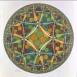 In Escher's picture Circle Limit III, 1959, the map from a given fish to the one in front of it is a hyperbolic transformation.
If α is zero (or a multiple of 2π), then the transformation is said to be hyperbolic. These transformations tend to move points along circular paths from one fixed point toward the other.
If we take the one-parameter subgroup generated by any hyperbolic Möbius transformation, we obtain a continuous transformation, such that every transformation in the subgroup fixes the same two points. All other points flow along a certain family of circular arcs away from the first fixed point and toward the second fixed point. In general, the two fixed points may be any two distinct points on the Riemann sphere.
This too has an important physical interpretation. Imagine that an observer accelerates (with constant magnitude of acceleration) in the direction of the North pole on his celestial sphere. Then the appearance of the night sky is transformed in exactly the manner described by the one-parameter subgroup of hyperbolic transformations sharing the fixed points
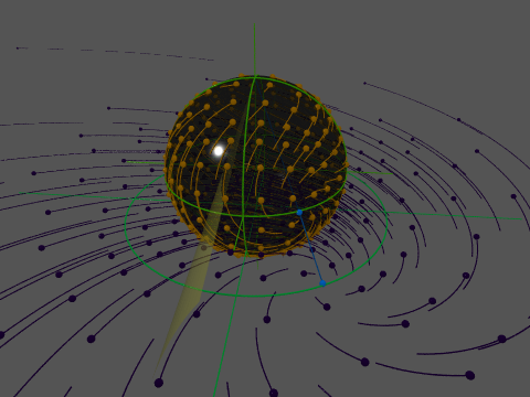
, with the real number ρ corresponding to the magnitude of his acceleration vector. The stars seem to move along longitudes, away from the South pole toward the North pole. (The longitudes appear as circular arcs under stereographic projection from the sphere to the plane).Here are some figures illustrating the effect of a hyperbolic Möbius transformation on the Riemann sphere (after stereographic projection to the plane):


These pictures resemble the field lines of a positive and a negative electrical charge located at the fixed points, because the circular flow lines subtend a constant angle between the two fixed points.
Loxodromic transformations
If both ρ and α are nonzero, then the transformation is said to be loxodromic. These transformations tend to move all points in S-shaped paths from one fixed point to the other.
The word "loxodrome" is from the Greek: "λοξος (loxos), slanting + δρόμος (dromos), course". When sailing on a constant bearing - if you maintain a heading of (say) north-east, you will eventually wind up sailing around the north pole in a logarithmic spiral. On the mercator projection such a course is a straight line, as the north and south poles project to infinity. The angle that the loxodrome subtends relative to the lines of longitude (i.e. its slope, the "tightness" of the spiral) is the argument of k. Of course, Möbius transformations may have their two fixed points anywhere, not just at the north and south poles. But any loxodromic transformation will be conjugate to a transform that moves all points along such loxodromes.
If we take the one-parameter subgroup generated by any loxodromic Möbius transformation, we obtain a continuous transformation, such that every transformation in the subgroup fixes the same two points. All other points flow along a certain family of curves, away from the first fixed point and toward the second fixed point. Unlike the hyperbolic case, these curves are not circular arcs, but certain curves which under stereographic projection from the sphere to the plane appear as spiral curves which twist counterclockwise infinitely often around one fixed point and twist clockwise infinitely often around the other fixed point. In general, the two fixed points may be any two distinct points on the Riemann sphere.
You can probably guess the physical interpretation in the case when the two fixed points are
: an observer who is both rotating (with constant angular velocity) about some axis and moving along the same axis, will see the appearance of the night sky transform according to the one-parameter subgroup of loxodromic transformations with fixed points , and with ρ,α determined respectively by the magnitude of the actual linear and angular velocities.Stereographic projection
These images show Möbius transformations stereographically projected onto the Riemann sphere. Note in particular that when projected onto a sphere, the special case of a fixed point at infinity looks no different from having the fixed points in an arbitrary location.
One fixed point at infinity  Elliptic
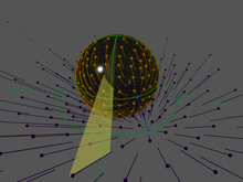 Hyperbolic
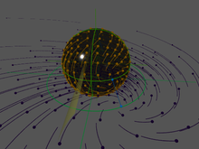 Loxodromic
Fixed points diametrically opposite 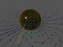 Elliptic
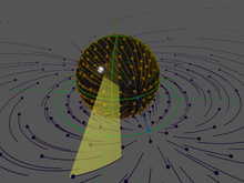 Hyperbolic
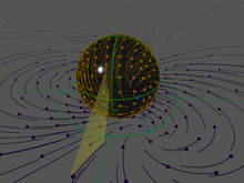 Loxodromic
Fixed points in an arbitrary location 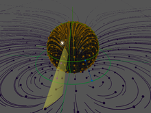 Elliptic
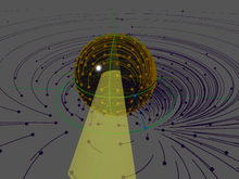 Hyperbolic
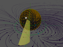 Loxodromic
Iterating a transformation
If a transformation
has fixed points γ1,γ2, and characteristic constant k, then  will have γ1' = γ1, γ2' = γ2, k' = kn.
This can be used to iterate a transformation, or to animate one by breaking it up into steps.
These images show three points (red, blue and black) continuously iterated under transformations with various characteristic constants.


And these images demonstrate what happens when you transform a circle under Hyperbolic, Elliptical, and Loxodromic transforms. Note that in the elliptical and loxodromic images, the α value is 1/10 .


Poles of the transformation
The point
is called the pole of
; it is that point which is transformed to the point at infinity under .The inverse pole
is that point to which the point at infinity is transformed. The point midway between the two poles is always the same as the point midway between the two fixed points:
These four points are the vertices of a parallelogram which is sometimes called the characteristic parallelogram of the transformation.
A transform
can be specified with two fixed points γ1,γ2 and the pole  .
.This allows us to derive a formula for conversion between k and
given γ1,γ2:which reduces down to
The last expression coincides with one of the (mutually reciprocal) eigenvalue ratios
 of the matrix
representing the transform (compare the discussion in the preceding section about the characteristic constant of a transformation). Its characteristic polynomial is equal to
which has roots
Lorentz transformations
The real Minkowski space consists of the four-dimensional real coordinate space R4 consisting of the space of ordered quadruples (x0,x1,x2,x3) of real numbers, together with a quadratic form
Borrowing terminology from special relativity, points with Q > 0 are considered timelike; in addition, if x0 > 0, then the point is called future-pointing. Points with Q < 0 are called spacelike. The null cone S consists of those points where Q = 0; the future null cone N+ are those points on the null cone with x0 > 0. The celestial sphere is then identified with the collection of rays in N+ whose initial point is the origin of R4. The collection of linear transformations on R4 with positive determinant preserving the quadratic form Q and preserving the time direction form the restricted Lorentz group SO+(1,3).
In connection with the geometry of the celestial sphere, the group of transformations SO+(1,3) is identified with the group PSL(2,C) of Möbius transformations of the sphere by exhibiting the action of the spin group on spinors (Penrose & Rindler 1986). To each (x0,x1,x2,x3) ∈ R4, associate the hermitian matrix
The determinant of the matrix X is equal to Q(x0,x1,x2,x3). The special linear group acts on the space of such matrices via
-

(
for each A ∈ SL(2,C), and this action of SL(2,C) preserves the determinant of X because det A = 1. Since the determinant of X is identified with the quadratic form Q, SL(2,C) acts by Lorentz transformations. On dimensional grounds, SL(2,C) covers a neighborhood of the identity of SO(1,3). Since SL(2,C) is connected, it covers the entire restricted Lorentz group SO+(1,3). Furthermore, if is that the kernel of the action (1) is the subgroup {±I}, then passing to the quotient group gives the group isomorphism
-

(
Focusing now attention on the case when (x0,x1,x2,x3) is null, the matrix X has zero determinant, and therefore splits as the outer product of a complex two-vector ξ with its complex conjugate:
-

(
The two-component vector ξ is acted upon by SL(2,C) in a manner compatible with (1). It is now clear that the kernel of the representation of SL(2,C) on hermitian matrices is {±I}.
The action of PSL(2,C) on the celestial sphere may also be described geometrically using stereographic projection. Consider first the hyperplane in R4 given by x0 = 1. The celestial sphere may be identified with the sphere S+ of intersection of the hyperplane with the future null cone N+. The stereographic projection from the north pole (1,0,0,1) of this sphere onto the plane x3 = 0 takes a point with coordinates (1,x1,x2,x3) with
to the point
Introducing the complex coordinate
the inverse stereographic projection gives the following formula for a point (x1, x2, x3) on S+:
-

(
The action of SO+(1,3) on the points of N+ does not preserve the hyperplane S+, but acting on points in S+ and then rescaling so that the result is again in S+ gives an action of SO+(1,3) on the sphere which goes over to an action on the complex variable ζ. In fact, this action is by fractional linear transformations, although this is not easily seen from this representation of the celestial sphere. Conversely, for any fractional linear transformation of ζ variable goes over to a unique Lorentz transformation on N+, possibly after a suitable (uniquely determined) rescaling.
A more invariant description of the stereographic projection which allows the action to be more clearly seen is to consider the variable ζ = z:w as a ratio of a pair of homogeneous coordinates for the complex projective line CP1. The stereographic projection goes over to a transformation from C2 − {0} to N+ which is homogeneous of degree two with respect to real scalings
-

(
which agrees with (4) upon restriction to scales in which
 The components of (5) are precisely those obtained from the outer product
In summary, the action of the restricted Lorentz group SO+(1,3) agrees with that of the Möbius group PSL(2,C). This motivates the following definition. In dimension n ≥ 2, the Möbius group Möb(n) is the group of all orientation-preserving conformal isometries of the round sphere Sn to itself. By realizing the conformal sphere as the space of future-pointing rays of the null cone in the Minkowski space R1,n+1, there is an isomorphism of Möb(n) with the restricted Lorentz group SO+(1,n+1) of Lorentz transformations with positive determinant, preserving the direction of time.
Hyperbolic space
As seen above, the Möbius group PSL(2,C) acts on Minkowski space as the group of those isometries that preserve the origin, the orientation of space and the direction of time. Restricting to the points where Q=1 in the positive light cone, which form a model of hyperbolic 3-space H 3, we see that the Möbius group acts on H 3 as a group of orientation-preserving isometries. In fact, the Möbius group is equal to the group of orientation-preserving isometries of hyperbolic 3-space.
If we use the Poincaré ball model, identifying the unit ball in R3 with H 3, then we can think of the Riemann sphere as the "conformal boundary" of H 3. Every orientation-preserving isometry of H 3 gives rise to a Möbius transformation on the Riemann sphere and vice versa; this is the very first observation leading to the AdS/CFT correspondence conjectures in physics.
Subgroups of the Möbius group
If we require the coefficients a, b, c, d of a Möbius transformation to be real numbers with ad - bc = 1, we obtain a subgroup of the Möbius group denoted as PSL(2,R). This is the group of those Möbius transformations that map the upper half-plane H = {x + iy : y > 0} to itself, and is equal to the group of all biholomorphic (or equivalently: bijective, conformal and orientation-preserving) maps H→H. If a proper metric is introduced, the upper half-plane becomes a model of the hyperbolic plane H 2, the Poincaré half-plane model, and PSL(2,R) is the group of all orientation-preserving isometries of H 2 in this model.
The subgroup of all Möbius transformations that map the open disk D = {z : |z| < 1} to itself consists of all transformations of the form
with
 ,
,  and | b | < 1. This is equal to the group of all biholomorphic (or equivalently: bijective, angle-preserving and orientation-preserving) maps D→D. By introducing a suitable metric, the open disk turns into another model of the hyperbolic plane, the Poincaré disk model, and this group is the group of all orientation-preserving isometries of H 2 in this model.
Since both of the above subgroups serve as isometry groups of H 2, they are isomorphic. A concrete isomorphism is given by conjugation with the transformation
which bijectively maps the open unit disk to the upper half plane.
Alternatively, consider an open disk with radius r, centered at ri. The Poincaré disk model in this disk becomes identical to the upper-half-plane model as r approaches ∞.
A maximal compact subgroup of the Möbius group
 is given by[1]
and corresponds under the isomorphism
 to the projective special unitary group
  which is isomorphic to the special orthogonal group
  of rotations in three dimensions, and can be interpreted as rotations of the Riemann sphere. Every finite subgroup is conjugate into this maximal compact group, and thus these correspond exactly to the polyhedral groups, the point groups in three dimensions.
Icosahedral groups of Möbius transformations were used by Felix Klein to give an analytic solution to the quintic equation in (Klein 1888); a modern exposition is given in.[2]
If we require the coefficients a, b, c, d of a Möbius transformation to be integers with ad - bc = 1, we obtain the modular group PSL(2,Z), a discrete subgroup of PSL(2,R) important in the study of lattices in the complex plane, elliptic functions and elliptic curves. The discrete subgroups of PSL(2,R) are known as Fuchsian groups; they are important in the study of Riemann surfaces.
See also
Notes
- ^ Geometrically this map is the stereographic projection of a rotation by 90° around with period 4, which takes

References
- Beardon, Alan F. (1995), The Geometry of Discrete Groups, New York: Springer-Verlag, ISBN 978-0-387-90788-8
- Hall, G. S. (2004), Symmetries and Curvature Structure in General Relativity, Singapore: World Scientific, ISBN 978-981-02-1051-9 (See Chapter 6 for the classification, up to conjugacy, of the Lie subalgebras of the Lie algebra of the Lorentz group.)
- Katok, Svetlana (1992), Fuchsian Groups, Chicago:University of Chicago Press, ISBN 978-0-226-42583-2 See Chapter 2.
- Klein, Felix (1888), Lectures on the ikosahedron and the solution of equations of the fifth degree, http://digital.library.cornell.edu/cgi/t/text/text-idx?c=math;cc=math;view=toc;subview=short;idno=03070001, Dover edition ISBN 978-0-486-49528-6.
- Knopp, Konrad (1952), Elements of the Theory of Functions, New York: Dover, ISBN 978-0-486-60154-0 (See Chapters 3-5 of this classic book for a beautiful introduction to the Riemann sphere, stereographic projection, and Möbius transformations.)
- Mumford, David; Series, Caroline; Wright, David (2002), Indra's Pearls: The Vision of Felix Klein, Cambridge University Press, ISBN 978-0-521-35253-6 (Aimed at non-mathematicians, provides an excellent exposition of theory and results, richly illustrated with diagrams.)
- Needham, Tristan (1997), Visual Complex Analysis, Oxford: Clarendon Press, ISBN 978-0-19-853446-4 (See Chapter 3 for a beautifully illustrated introduction to Möbius transformations, including their classification up to conjugacy.)
- Penrose, Roger; Rindler, Wolfgang (1986), Spinors and space-time, Volume 1: Two-spinor calculus and relativistic fields, Cambridge University Press, ISBN 978-0-521-24527-2
- Tóth, Gábor (2002), Finite Möbius groups, minimal immersions of spheres, and moduli
External links
- A java applet allowing you to specify a transformation via its fixed points and so on.
- A java applet demonstrating iterated application of a Möbius transformation to a circle.
- Conformal maps gallery
- Weisstein, Eric W., "Linear Fractional Transformation" from MathWorld.
- Möbius Transformation Module by John H. Mathews
- Linear Fractional Transformations at MathPages
- Möbius Transformations Revealed, by Douglas N. Arnold and Jonathan Rogness (a video by two University of Minnesota professors explaining and illustrating Möbius transformations using stereographic projection from a sphere). A high resolution version in QuickTime format is available at http://www.ima.umn.edu/~arnold/moebius/index.html .
Categories:- Projective geometry
- Continued fractions
- Conformal geometry
- Lie groups
- Riemann surfaces
- Functions and mappings
- Kleinian groups


![[z_1 : z_2]\leftrightarrow z_1/z_2.](5/0d5cef6faf5445861e5c9d7264c11a7c.png)


Wikimedia Foundation. 2010.