- Miller effect
-
In electronics, the Miller effect accounts for the increase in the equivalent input capacitance of an inverting voltage amplifier due to amplification of the effect of capacitance between the input and output terminals. The virtually increased input capacitance due to the Miller effect is given by
where − Av is the gain of the amplifier and C is the feedback capacitance.
Although the term Miller effect normally refers to capacitance, any impedance connected between the input and another node exhibiting gain can modify the amplifier input impedance via this effect. These properties of the Miller effect are generalized in the Miller theorem.
Contents
History
The Miller effect was named after John Milton Miller.[1] When Miller published his work in 1920, he was working on vacuum tube triodes, however the same theory applies to more modern devices such as bipolar and MOS transistors.
Derivation
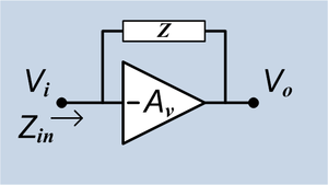 An ideal voltage inverting amplifier with an impedance connecting output to input.
Consider an ideal inverting voltage amplifier of gain − Av with an impedance Z connected between its input and output nodes. The output voltage is therefore Vo = − AvVi. Assuming that the amplifier input draws no current, all of the input current flows through Z, and is therefore given by
 .
.
The input impedance of the circuit is
If Z represents a capacitor with impedance
 , the resulting input impedance is
Thus the effective or Miller capacitance CM is the physical C multiplied by the factor (1 + Av)[2].
Effects
As most amplifiers are inverting (i.e. Av < 0), the effective capacitance at their inputs is increased due to the Miller effect. This can lower the bandwidth of the amplifier, reducing its range of operation to lower frequencies. The tiny junction and stray capacitances between the base and collector terminals of a Darlington transistor, for example, may be drastically increased by the Miller effects due to its high gain, lowering the high frequency response of the device.
It is also important to note that the Miller capacitance is the capacitance seen looking into the input. If looking for all of the RC time constants (poles) it is important to include as well the capacitance seen by the output. The capacitance on the output is often neglected since it sees C(1 − 1 / Av) and amplifier outputs are typically low impedance. However if the amplifier has a high impedance output, such as if a gain stage is also the output stage, then this RC can have a significant impact on the performance of the amplifier. This is when pole splitting techniques are used.
The Miller effect may also be exploited to synthesize larger capacitors from smaller ones. One such example is in the stabilization of feedback amplifiers, where the required capacitance may be too large to practically include in the circuit. This may be particularly important in the design of integrated circuit, where capacitors can consume significant area, increasing costs.
Mitigation
The Miller effect may be undesired in many cases, and approaches may be sought to lower its impact. Several such techniques are used in the design of amplifiers.
A current buffer stage may be added at the output to lower the gain Av between the input and output terminals of the amplifier (though not necessarily the overall gain). For example, a common base may be used as a current buffer at the output of a common emitter stage, forming a cascode. This will typically reduce the Miller effect and increase the bandwidth of the amplifier.
Alternatively, a voltage buffer may be used before the amplifier input, reducing the effective source impedance seen by the input terminals. This lowers the RC time constant of the circuit and typically increases the bandwidth.
Impact on frequency response
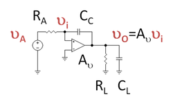 Figure 2: Operational amplifier with feedback capacitor CC.
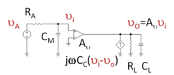 Figure 3: Circuit of Figure 2 transformed using Miller's theorem, introducing the Miller capacitance on the input side of the circuit.
Figure 2 shows an example of Figure 1 where the impedance coupling the input to the output is the coupling capacitor CC. A Thévenin voltage source VA drives the circuit with Thévenin resistance RA. At the output a parallel RC-circuit serves as load. (The load is irrelevant to this discussion: it just provides a path for the current to leave the circuit.) In Figure 2, the coupling capacitor delivers a current jωCC( vi - vo ) to the output node.
Figure 3 shows a circuit electrically identical to Figure 2 using Miller's theorem. The coupling capacitor is replaced on the input side of the circuit by the Miller capacitance CM, which draws the same current from the driver as the coupling capacitor in Figure 2. Therefore, the driver sees exactly the same loading in both circuits. On the output side, a dependent current source in Figure 3 delivers the same current to the output as does the coupling capacitor in Figure 2. That is, the R-C-load sees the same current in Figure 3 that it does in Figure 2.
In order that the Miller capacitance draw the same current in Figure 3 as the coupling capacitor in Figure 2, the Miller transformation is used to relate CM to CC. In this example, this transformation is equivalent to setting the currents equal, that is
or, rearranging this equation
This result is the same as CM of the Derivation Section.
The present example with Av frequency independent shows the implications of the Miller effect, and therefore of CC, upon the frequency response of this circuit, and is typical of the impact of the Miller effect (see, for example, common source). If CC = 0 F, the output voltage of the circuit is simply Av vA, independent of frequency. However, when CC is not zero, Figure 3 shows the large Miller capacitance appears at the input of the circuit. The voltage output of the circuit now becomes
and rolls off with frequency once frequency is high enough that ω CMRA ≥ 1. It is a low-pass filter. In analog amplifiers this curtailment of frequency response is a major implication of the Miller effect. In this example, the frequency ω3dB such that ω3dB CMRA = 1 marks the end of the low-frequency response region and sets the bandwidth or cutoff frequency of the amplifier.
It is important to notice that the effect of CM upon the amplifier bandwidth is greatly reduced for low impedance drivers (CM RA is small if RA is small). Consequently, one way to minimize the Miller effect upon bandwidth is to use a low-impedance driver, for example, by interposing a voltage follower stage between the driver and the amplifier, which reduces the apparent driver impedance seen by the amplifier.
The output voltage of this simple circuit is always Av vi. However, real amplifiers have output resistance. If the amplifier output resistance is included in the analysis, the output voltage exhibits a more complex frequency response and the impact of the frequency-dependent current source on the output side must be taken into account.[3] Ordinarily these effects show up only at frequencies much higher than the roll-off due to the Miller capacitance, so the analysis presented here is adequate to determine the useful frequency range of an amplifier dominated by the Miller effect.
Miller approximation
This example also assumes Av is frequency independent, but more generally there is frequency dependence of the amplifier contained implicitly in Av. Such frequency dependence of Av also makes the Miller capacitance frequency dependent, so interpretation of CM as a capacitance becomes more difficult. However, ordinarily any frequency dependence of Av arises only at frequencies much higher than the roll-off with frequency caused by the Miller effect, so for frequencies up to the Miller-effect roll-off of the gain, Av is accurately approximated by its low-frequency value. Determination of CM using Av at low frequencies is the so-called Miller approximation.[2] With the Miller approximation, CM becomes frequency independent, and its interpretation as a capacitance at low frequencies is secure.
References and notes
- ^ John M. Miller, "Dependence of the input impedance of a three-electrode vacuum tube upon the load in the plate circuit," Scientific Papers of the Bureau of Standards, vol.15, no. 351, pages 367-385 (1920). Available on-line at: http://web.mit.edu/klund/www/papers/jmiller.pdf .
- ^ a b R.R. Spencer and M.S. Ghausi (2003). Introduction to electronic circuit design.. Upper Saddle River NJ: Prentice Hall/Pearson Education, Inc.. p. 533. ISBN 0-201-36183-3. http://worldcat.org/isbn/0-201-36183-3.
- ^ See article on pole splitting.
See also
Categories:- Electronics terms
- Electrical engineering
- Electronic design
- Analog circuits


Wikimedia Foundation. 2010.