Permanent is sharp-P-complete

The correct title of this article is Permanent is #P-complete. The substitution or omission of the # sign is because of technical restrictions.

In a 1979 paper Leslie Valiant proved^[1] that the problem of computing the permanent of a matrix is #P-hard, and remains #P-complete even if the matrix is restricted to have entries that are all 0 or 1. This result is sometimes known as Valiant's theorem^[2] and is considered a seminal result in computational complexity theory.^[3][4] Valiant's 1979 paper also introduced #P as a complexity class.^[5]

Significance

One reason for interest in the computational complexity of the permanent is that it provides an example of a problem where constructing a single solution can be done efficiently but where counting all solutions is hard.^[6] As Papadimitriou writes in his book Computational Complexity:

“

The most impressive and interesting #P-complete problems are those for which the corresponding search problem can be solved in polynomial time. The PERMANENT problem for 0–1 matrices, which is equivalent to the problem of counting perfect matchings in a bipartite graph [...] is the classic example here.[2]

”

Specifically, computing the permanent (shown to be difficult by Valiant's results) is closely connected with finding a perfect matching in a bipartite graph, which is solvable in polynomial time by the Hopcroft–Karp algorithm.^[7][8] For a bipartite graph with 2n vertices partitioned into two parts with n vertices each, the number of perfect matchings equals the permanent of its biadjacency matrix and the square of the number of perfect matchings is equal to the permanent of its adjacency matrix.^[9] Since any 0–1 matrix is the biadjacency matrix of some bipartite graph, Valiant's theorem implies^[9] that the problem of counting the number of perfect matchings in a bipartite graph is #P-complete, and in conjunction with Toda's theorem this implies that it is hard for the entire polynomial hierarchy.^[10][11]

The computational complexity of the permanent also has some significance in other aspects of complexity theory: it is not known whether NC equals P (informally, whether every polynomially-solvable problem can be solved by a polylogarithmic-time parallel algorithm) and Ketan Mulmuley has suggested an approach to resolving this question that relies on writing the permanent as the determinant of a matrix.^{[citation needed]}

Hartmann ^[12] proved a generalization of Valiant's theorem concerning the complexity of computing immanants of matrices that generalize both the determinant and the permanent.

Ben-Dor and Halevi's proof

Below, the proof that computing the permanent of a 01-matrix is #P-complete is described. It mainly follows the proof by Ben-Dor & Halevi (1993).^[13]

Overview

Any square matrix A = (a_ij) can be viewed as the adjacency matrix of a directed graph, with a_ij representing the weight of the edge from vertex i to vertex j. Then, the permanent of A is equal to the sum of the weights of all cycle-covers of the graph; this is a graph-theoretic interpretation of the permanent.

#SAT, a function problem related to the Boolean satisfiability problem, is the problem of counting the number of satisfying assignments of a given Boolean formula. It is a #P-complete problem (by definition), as any NP machine can be encoded into a Boolean formula by a process similar to that in Cook's theorem, such that the number of satisfying assignments of the Boolean formula is equal to the number of accepting paths of the NP machine. Any formula in SAT can be rewritten as a formula in 3-CNF form preserving the number of satisfying assignments, and so #SAT and #3SAT are equivalent and #3SAT is #P-complete as well.

In order to prove that 01-Permanent is #P-hard, it is therefore sufficient to show that the number of satisfying assignments for a 3-CNF formula can be expressed succinctly as a function of the permanent of a matrix that contains only the values 0 and 1. This is usually accomplished in two steps:

1. Given a 3-CNF formula φ, construct a directed integer-weighted graph G_ϕ, such that the sum of the weights of cycle covers of G_ϕ (or equivalently, the permanent of its adjacency matrix) is equal to the number of satisfying assignments of φ. This establishes that Permanent is #P-hard.
2. Through a series of reductions, reduce Permanent to 01-Permanent, the problem of computing the permanent of a matrix all entries 0 or 1. This establishes that 01-permanent is #P-hard as well.

Constructing the integer graph

Given a 3CNF-formula ϕ with m clauses and n variables, one can construct a weighted, directed graph G_ϕ such that

1. each satisfying assignment for ϕ will have a corresponding set of cycle covers in G_ϕ where the sum of the weights of cycle covers in this set will be 12^m ; and
2. all other cycle covers in G_ϕ will have weights summing to 0.

Thus if $(\#\phi)$ is the number of satisfying assignments for ϕ, the permanent of this graph will be $12^m \cdot (\#\phi)$. (Valiant's original proof constructs a graph with entries in { − 1,0,1,2,3} whose permanent is $4^{t(\phi)}\cdot(\#\phi)$ where t(ϕ) is "twice the number of occurrences of literals in ϕ" – m.)

The graph construction makes use of a component that is treated as a "black box." To keep the explanation simple, the properties of this component are given without actually defining the structure of the component.

To specify G_φ, one first constructs a variable node in G_φ for each of the n variables in φ. Additionally, for each of the m clauses in φ, one constructs a clause component C_j in G_φ that functions as a sort of "black box." All that needs to be noted about C_j is that it has three input edges and three output edges. The input edges come either from variable nodes or from previous clause components (e.g., C_o for some o < j) and the output edges go either to variable nodes or to later clause components (e.g., C_o for some o > j). The first input and output edges correspond with the first variable of the clause j, and so on. Thus far, all of the nodes that will appear in the graph G_φ have been specified.

Next, one would consider the edges. For each variable x_i of ϕ, one makes a true cycle (T-cycle) and a false cycle (F-cycle) in G_ϕ. To create the T-cycle, one starts at the variable node for x_i and draw an edge to the clause component C_j that corresponds to the first clause in which x_i appears. If x_i is the first variable in the clause of ϕ corresponding to C_j, this edge will be the first input edge of C_j, and so on. Thence, draw an edge to the next clause component corresponding to the next clause of ϕ in which x_i appears, connecting it from the appropriate output edge of C_j to the appropriate input edge of the next clause component, and so on. After the last clause in which x_i appears, we connect the appropriate output edge of the corresponding clause component back to x_i's variable node. Of course, this completes the cycle. To create the F-cycle, one would follow the same procedure, but connect x_i's variable node to those clause components in which ~x_i appears, and finally back to x_i's variable node. All of these edges outside the clause components are termed external edges, all of which have weight 1. Inside the clause components, the edges are termed internal edges. Every external edge is part of a T-cycle or an F-cycle (but not both—that would force inconsistency).

Note that the graph G_ϕ is of size linear in | ϕ | , so the construction can be done in polytime (assuming that the clause components do not cause trouble).

Notable properties of the graph

A useful property of G_ϕ is that its cycle covers correspond to variable assignments for ϕ. For a cycle cover Z of G_ϕ, one can say that Z induces an assignment of values for the variables in ϕ just in case Z contains all of the external edges in x_i's T-cycle and none of the external edges in x_i's F-cycle for all variables x_i that the assignment makes true, and vice versa for all variables x_i that the assignment makes false. Although any given cycle cover Z need not induce an assignment for ϕ, any one that does induces exactly one assignment, and the same assignment induced depends only on the external edges of Z. The term Z is considered an incomplete cycle cover at this stage, because one talks only about its external edges, M. In the section below, one considers M-completions to show that one has a set of cycle covers corresponding to each M that have the necessary properties.

The sort of Z's that don't induce assignments are the ones with cycles that "jump" inside the clause components. That is, if for every C_j, at least one of C_j's input edges is in Z, and every output edge of the clause components is in Z when the corresponding input edge is in Z, then Z is proper with respect to each clause component, and Z will produce a satisfying assignment for ϕ. This is because proper Z's contain either the complete T-cycle or the complete F-cycle of every variable x_i in ϕ as well as each including edges going into and coming out of each clause component. Thus, these Z's assign either true or false (but never both) to each x_i and ensure that each clause is satisfied. Further, the sets of cycle covers corresponding to all such Z's have weight 12^m, and any other Z's have weight 0. The reasons for this depend on the construction of the clause components, and are outlined below.

The clause component

To understand the relevant properties of the clause components C_j, one needs the notion of an M-completion. A cycle cover Z induces a satisfying assignment just in case its external edges satisfy certain properties. For any cycle cover of G_ϕ, consider only its external edges, the subset M. Let M be a set of external edges. A set of internal edges L is an M-completion just in case $M\cup L$ is a cycle cover of G_ϕ. Further, denote the set of all M-completions by L^M and the set of all resulting cycle covers of G_ϕ by Z^M.

Recall that construction of G_ϕ was such that each external edge had weight 1, so the weight of Z^M, the cycle covers resulting from any M, depends only on the internal edges involved. We add here the premise that the construction of the clause components is such that the sum over possible M-completions of the weight of the internal edges in each clause component, where M is proper relative to the clause component, is 12. Otherwise the weight of the internal edges is 0. Since there are m clause components, and the selection of sets of internal edges, L, within each clause component is independent of the selection of sets of internal edges in other clause components, so one can multiply everything to get the weight of Z^M. So, the weight of each Z^M, where M induces a satisfying assignment, is 12^m. Further, where M does not induce a satisfying assignment, M is not proper with respect to some C_j, so the product of the weights of internal edges in Z^M will be 0.

The clause component is a weighted, directed graph with 7 nodes with edges weighted and nodes arranged to yield the properties specified above, and is given in Appendix A of Ben-Dor and Halevi (1993). Note that the internal edges here have weights drawn from the set { − 1,0,1,2,3}; not all edges have 0–1 weights.

Finally, since the sum of weights of all the sets of cycle covers inducing any particular satisfying assignment is 12^m, and the sum of weights of all other sets of cycle covers is 0, one has Perm(G_φ) = 12^m·(#φ). The following section reduces computing Perm(G_ϕ) to the permanent of a 01 matrix.

01-Matrix

The above section has shown that Permanent is #P-hard. Through a series of reductions, any permanent can be reduced to the permanent of a matrix with entries only 0 or 1. This will prove that 01-Permanent is #P-hard as well.

Reduction to a non-negative matrix

Using modular arithmetic, convert an integer matrix A into an equivalent non-negative matrix A' so that the permanent of A can be computed easily from the permanent of A', as follows:

Let A be an $n \times n$ integer matrix where no entry has a magnitude larger than μ.

• Compute $Q = 2 n! \cdot \mu^n + 1$. The choice of Q is due to the fact that $|\operatorname{Perm}(A)| \le n! \cdot \mu^n$
• Compute $A' = A\,\bmod\,Q$
• Compute $P = \operatorname{Perm}(A')\,\bmod\,Q$
• If P < Q / 2 then Perm(A) = P. Otherwise Perm(A) = P − Q

The transformation of A into A' is polynomial in n and log(μ), since the number of bits required to represent Q is polynomial in n and log(μ)

An example of the transformation and why it works is given below.

$A = \begin{bmatrix}2 & -2 \\ -2 & 1\end{bmatrix}$

$\operatorname{Perm}(A) = 2 \cdot 1 + (-2) \cdot (-2) = 6$.

Here, n = 2, μ = 2, and μⁿ = 4, so Q = 17. Thus

$A' = A\,\bmod\,17 = \begin{bmatrix}2 & 15 \\ 15 & 1\end{bmatrix}.$

Note how the elements are non-negative because of the modular arithmetic. It is simple to compute the permanent

$\operatorname{Perm}(A') = 2 \cdot 1 + 15 \cdot 15 = 227$

so $P = 227\,\bmod\,17 = 6$. Then P < Q / 2, so $\operatorname{Perm}(A) = P = 6.$

Reduction to powers of 2

Note that any number can be decomposed into a sum of powers of 2. For example,

13 = 2³ + 2² + 2⁰

This fact is used to convert a non-negative matrix into an equivalent matrix whose entries are all powers of 2. The reduction can be expressed in terms of graphs equivalent to the matrices.

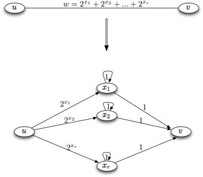
Let G be a n-node weighted directed graph with non-negative weights, where largest weight is W. Every edge e with weight w is converted into an equivalent edge with weights in powers of 2 as follows:

$w = 2^{x_1} + 2^{x_2} + \cdots + 2^{x_r}$, $0 \le x_1 \le x_2 \le \cdots \le x_r \le \log (w)$

This can be seen graphically in the Figure 1. The subgraph that replaces the existing edge contains r nodes and 3r edges.

To prove that this produces an equivalent graph G' that has the same permanent as the original, one must show the correspondence between the cycle covers of G and G'.

Consider some cycle-cover R in G.

• If an edge e is not in R, then to cover all the nodes in the new sub graph, one must use the self-loops. Since all self-loops have a weight of 1, the weight of cycle-covers in R and R' match.
• If e is in R, then in all the corresponding cycle-covers in G', there must be a path from u to v, where u and v are the nodes of edge e. From the construction, one can see that there are r different paths and sum of all these paths equal to the weight of the edge in the original graph G. So the weight of corresponding cycle-covers in G and G' match.

Note that the size of G' is polynomial in n and log W.

Reduction to 0–1

The objective here is to reduce a matrix whose entries are powers of 2 into an equivalent matrix containing only zeros and ones (i.e. a directed graph where each edge has a weight of 1).

Let G be a n-node directed graph where all the weights on edges are powers of two. Construct a graph, G', where the weight of each edge is 1 and Perm(G) = Perm(G'). The size of this new graph, G', is polynomial in n and p where the maximal weight of any edge in graph G is 2^p.

This reduction is done locally at each edge in G that has a weight larger than 1. Let e = (u,v) be an edge in G with a weight w = 2^r > 1. It is replaced by a subgraph J_e that is made up of 2r nodes and 6r edges as seen in Figure 2. Each edge in J_e has a weight of 1. Thus, the resulting graph G' contains only edges with a weight of 1.

Consider some cycle-cover R in G.

• If an original edge e from graph G is not in R, one cannot create a path through the new subgraph J_e. The only way to form a cycle cover over J_e in such a case is for each node in the subgraph to take its self-loop. As each edge has a weight of one, the weight of the resulting cycle cover is equal to that of the original cycle cover.
• However, if the edge in G is a part of the cycle cover then in any cycle cover of G' there must be a path from u to v in the subgraph. At each step down the subgraph there are two choices one can make to form such a path. One must make this choice r times, resulting in 2^r possible paths from u to v. Thus, there are 2^r possible cycle covers and since each path has a weight of 1, the sum of the weights of all these cycle covers equals the weight of the original cycle cover.

References

1. ^ Leslie G. Valiant (1979). "The Complexity of Computing the Permanent". Theoretical Computer Science (Elsevier) 8 (2): 189–201. doi:10.1016/0304-3975(79)90044-6. 
2. ^ ^{a b} Christos H. Papadimitriou. Computational Complexity. Addison-Wesley, 1994. ISBN 0-201-53082-1. Page 443
3. ^ Allen Kent, James G. Williams, Rosalind Kent and Carolyn M. Hall (editors). Encyclopedia of microcomputers.Marcel Dekker, 1999. ISBN 978-0-8247-2722-2; p. 34
4. ^ Jin-Yi Cai, A. Pavan and D. Sivakumar, On the Hardness of Permanent. In: STACS, '99: 16th Annual Symposium on Theoretical Aspects of Computer Science, Trier, Germany, March 4–6, 1999 Proceedings. pp. 90–99. Springer-Verlag, New York, LLC Pub. Date: October 2007. ISBN 978-3-540-65691-3; p. 90.
5. ^ L. Fortnow. My Favorite Ten Complexity Theorems of the Past Decade. Foundations of Software Technology and Theoretical Computer Science: Proceedings of the 14th Conference, Madras, India, December 15–17, 1994. P. S. Thiagarajan (editor), pp. 256–275, Springer-Verlag, New York, 2007. ISBN 978-3-540-58715-6; p. 265
6. ^ Peter Burgisser.Completeness and Reduction in Algebraic Complexity Theory. Springer-Verlag, New York, 2000. ISBN 978-3-540-66752-0; p. 2
7. ^ John E. Hopcroft, Richard M. Karp: An n^{5 / 2} Algorithm for Maximum Matchings in Bipartite Graphs. SIAM J. Comput. 2(4), 225–231 (1973)
8. ^ Cormen, Thomas H.; Leiserson, Charles E., Rivest, Ronald L., Stein, Clifford (2001) [1990]. "26.5: The relabel-to-front algorithm". Introduction to Algorithms (2nd ed.). MIT Press and McGraw-Hill. pp. pp. 696–697. ISBN 0-262-03293-7. 
9. ^ ^{a b} Dexter Kozen. The Design and Analysis of Algorithms. Springer-Verlag, New York, 1991. ISBN 978-0-387-97687-7; pp. 141–142
10. ^ Seinosuke Toda. PP is as Hard as the Polynomial-Time Hierarchy. SIAM Journal on Computing, Volume 20 (1991), Issue 5, pp. 865–877.
11. ^ 1998 Gödel Prize. Seinosuke Toda
12. ^ W. Hartmann. On the complexity of immanants. Linear and Multilinear Algebra 18 (1985), no. 2, pp. 127–140.
13. ^ Ben-Dor, Amir; Halevi, Shai (1993). "Proceedings of the 2nd Israel Symposium on the Theory and Computing Systems". pp. 108–117. http://citeseer.ist.psu.edu/ben-dor95zeroone.html. .