Radioactive decay

For particle decay in a more general context, see Particle decay. For more information on hazards of various kinds of radiation from decay, see Ionizing radiation.

"Radioactive" redirects here. For other uses, see Radioactive (disambiguation).

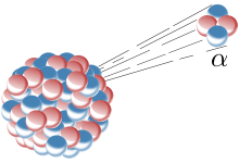Alpha decay is one example type of radioactive decay, in which an atomic nucleus emits an alpha particle, and thereby transforms (or 'decays') into an atom with a mass number 4 less and atomic number 2 less. Many other types of decays are possible.

Radioactive decay is the process by which an atomic nucleus of an unstable atom loses energy by emitting ionizing particles (ionizing radiation). The emission is spontaneous, in that the atom decays without any physical interaction with another particle from outside the atom. Usually, radioactive decay happens due to a process confined to the nucleus of the unstable atom, but, on occasion (as with the different processes of electron capture and internal conversion), an inner electron of the radioactive atom is also necessary to the process.

Radioactive decay is a stochastic (i.e., random) process at the level of single atoms, in that, according to quantum theory, it is impossible to predict when a given atom will decay.^[1] However, the chance that a given atom will decay is constant over time. For a large number of identical atoms (of the same nuclide), the decay rate for the collection is predictable to the extent allowed by the law of large numbers, and is easily calculated from the measured decay constant of the nuclide (or equivalently from the half-life).

The decay, or loss of energy, results when an atom with one type of nucleus, called the parent radionuclide, transforms to an atom with a nucleus in a different state, or a different nucleus, either of which is named the daughter nuclide. Often the parent and daughter are different chemical elements, and in such cases the decay process results in nuclear transmutation. In an example of this, a carbon-14 atom (the "parent") emits radiation (a beta particle, antineutrino, and a gamma ray) and transforms to a nitrogen-14 atom (the "daughter"). By contrast, there exist two types of radioactive decay processes (gamma decay and internal conversion decay) that do not result in transmutation, but only decrease the energy of an excited nucleus. This results in an atom of the same element as before but with a nucleus in a lower energy state. An example is the nuclear isomer technetium-99m decaying, by the emission of a gamma ray, to an atom of technetium-99.

Nuclides produced by radioactive decay are called radiogenic nuclides, whether they themselves are stable or not. There exist stable radiogenic nuclides that were formed from short-lived extinct radionuclides in the early solar system^{[citation needed]}. The extra presence of stable radiogenic nuclides against the background of primordial stable nuclides can be inferred by various means. Presently-radioactive nuclides are from three sources: many naturally-occurring radionuclides are short-lived radiogenic nuclides that are the daughters of ongoing radioactive primordial nuclides (types of radioactive atoms that have been present since the beginning of the Earth and solar system). Other naturally-occurring radioactive nuclides are cosmogenic nuclides, formed by cosmic ray bombardment of material in the Earth's atmosphere or crust. Finally, some primordial nuclides are radioactive, but are so long-lived that they remain present from the primordial solar nebula. For a summary table showing the number of stable nuclides and of radioactive nuclides in each category, see radionuclide.

The SI unit of activity is the becquerel (Bq). One Bq is defined as one transformation (or decay) per second. Since any reasonably-sized sample of radioactive material contains many atoms, a Bq is a tiny measure of activity; amounts on the order of GBq (gigabecquerel, 1 x 10⁹ decays per second) or TBq (terabecquerel, 1 x 10¹² decays per second) are commonly used. Another unit of radioactivity is the curie, Ci, which was originally defined as the amount of radium emanation (radon-222) in equilibrium with one gram of pure radium, isotope Ra-226. At present it is equal, by definition, to the activity of any radionuclide decaying with a disintegration rate of 3.7 × 10¹⁰ Bq. The use of Ci is currently discouraged by the SI.

Explanation

The trefoil symbol is used to indicate radioactive material.

The neutrons and protons that constitute nuclei, as well as other particles that approach close enough to them, are governed by several interactions. The strong nuclear force, not observed at the familiar macroscopic scale, is the most powerful force over subatomic distances. The electrostatic force is almost always significant, and, in the case of beta decay, the weak nuclear force is also involved.

The interplay of these forces produces a number of different phenomena in which energy may be released by rearrangement of particles in the nucleus or the change of one particle into others. The rearrangement is hindered energetically, so that it does not occur immediately. Random quantum vacuum fluctuations are theorized to promote relaxation to a lower energy state (the "decay") in a phenomenon known as quantum tunneling.

One might draw an analogy with a snowfield on a mountain: While friction between the ice crystals may be supporting the snow's weight, the system is inherently unstable with regard to a state of lower potential energy. A disturbance would thus facilitate the path to a state of greater entropy: The system will move towards the ground state, producing heat, and the total energy will be distributable over a larger number of quantum states. Thus, an avalanche results. The total energy does not change in this process, but, because of the law of entropy, avalanches happen only in one direction and that is toward the "ground state" — the state with the largest number of ways in which the available energy could be distributed.

Such a collapse (a decay event) requires a specific activation energy. For a snow avalanche, this energy comes as a disturbance from outside the system, although such disturbances can be arbitrarily small. In the case of an excited atomic nucleus, the arbitrarily small disturbance comes from quantum vacuum fluctuations. A radioactive nucleus (or any excited system in quantum mechanics) is unstable, and can, thus, spontaneously stabilize to a less-excited system. The resulting transformation alters the structure of the nucleus and results in the emission of either a photon or a high-velocity particle that has mass (such as an electron, alpha particle, or other type).

Discovery

Radioactivity was first discovered during 1896 by the French scientist Henri Becquerel, while working on phosphorescent materials. These materials glow in the dark after exposure to light, and he suspected that the glow produced in cathode ray tubes by X-rays might be associated with phosphorescence. He wrapped a photographic plate in black paper and placed various phosphorescent salts on it. All results were negative until he used uranium salts. The result with these compounds was a blackening of the plate. These radiations were called Becquerel Rays.

It soon became clear that the blackening of the plate did not have anything to do with phosphorescence, because the plate blackened when the mineral was in the dark. Non-phosphorescent salts of uranium and metallic uranium also blackened the plate. It was clear that there is a form of radiation that could pass through paper that was causing the plate to become black.

At first it seemed that the new radiation was similar to the then recently-discovered X-rays. Further research by Becquerel, Ernest Rutherford, Paul Villard, Pierre Curie, Marie Curie, and others discovered that this form of radioactivity was significantly more complicated. Different types of decay can occur, producing very different types of radiation. Rutherford was the first to realize that they all occur with the same mathematical exponential formula (see below), and to realize that many decay processes resulted in the transmutation of one element to another.

The early researchers also discovered that many other chemical elements besides uranium have radioactive isotopes. A systematic search for the total radioactivity in uranium ores also guided Marie Curie to isolate a new element polonium and to separate a new element radium from barium. The two elements' chemical similarity would otherwise have made them difficult to distinguish.

Danger of radioactive substances

Main article: Ionizing radiation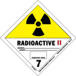

The danger classification sign of radioactive materials

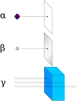Alpha particles may be completely stopped by a sheet of paper, beta particles by aluminum shielding. Gamma rays can only be reduced by much more substantial barriers, such as a very thick layer of lead.

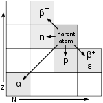Different types of decay of a radionuclide. Vertical: atomic number Z, Horizontal: neutron number N

The dangers of radioactivity and radiation were not immediately recognized. Acute effects of radiation were first observed in the use of X-rays when electrical engineer and physicist Nikola Tesla intentionally subjected his fingers to X-rays during 1896.^[2] He published his observations concerning the burns that developed, though he attributed them to ozone rather than to X-rays. His injuries healed later.

The genetic effects of radiation, including the effect on cancer risk, were recognized much later. During 1927, Hermann Joseph Muller published research showing genetic effects, and in 1946 was awarded the Nobel prize for his findings.

Before the biological effects of radiation were known, many physicians and corporations had begun marketing radioactive substances as patent medicine, glow-in-the-dark pigments, and radioactive quackery. Examples were radium enema treatments, and radium-containing waters to be drunk as tonics. Marie Curie protested this sort of treatment, warning that the effects of radiation on the human body were not well understood (Curie later died from aplastic anemia, which was likely caused by exposure to ionizing radiation). By the 1930s, after a number of cases of bone necrosis and death in enthusiasts, radium-containing medical products had been largely removed from the market.

Types of decay

As for types of radioactive radiation, it was found that an electric or magnetic field could split such emissions into three types of beams. For lack of better terms, the rays were given the alphabetic names alpha, beta, and gamma, still in use today. While alpha decay was seen only in heavier elements (atomic number 52, tellurium, and greater), the other two types of decay were seen in all of the elements.

In analyzing the nature of the decay products, it was obvious from the direction of electromagnetic forces produced upon the radiations by external magnetic and electric fields that alpha rays carried a positive charge, beta rays carried a negative charge, and gamma rays were neutral. From the magnitude of deflection, it was clear that alpha particles were much more massive than beta particles. Passing alpha particles through a very thin glass window and trapping them in a discharge tube allowed researchers to study the emission spectrum of the resulting gas, and ultimately prove that alpha particles are helium nuclei. Other experiments showed the similarity between classical beta radiation and cathode rays: They are both streams of electrons. Likewise gamma radiation and X-rays were found to be similar high-energy electromagnetic radiation.

The relationship between types of decays also began to be examined: For example, gamma decay was almost always found associated with other types of decay, occurring at about the same time, or afterward. Gamma decay as a separate phenomenon (with its own half-life, now termed isomeric transition), was found in natural radioactivity to be a result of the gamma decay of excited metastable nuclear isomers, in turn created from other types of decay.

Although alpha, beta, and gamma were found most commonly, other types of decay were eventually discovered. Shortly after the discovery of the positron in cosmic ray products, it was realized that the same process that operates in classical beta decay can also produce positrons (positron emission). In an analogous process, instead of emitting positrons and neutrinos, some proton-rich nuclides were found to capture their own atomic electrons (electron capture), and emit only a neutrino (and usually also a gamma ray). Each of these types of decay involves the capture or emission of nuclear electrons or positrons, and acts to move a nucleus toward the ratio of neutrons to protons that has the least energy for a given total number of nucleons (neutrons plus protons).

Shortly after discovery of the neutron in 1932, it was discovered by Enrico Fermi that certain rare decay reactions yield neutrons as a decay particle (neutron emission). Isolated proton emission was eventually observed in some elements. It was also found that some heavy elements may undergo spontaneous fission into products that vary in composition. In a phenomenon called cluster decay, specific combinations of neutrons and protons (atomic nuclei) other than alpha particles (helium nuclei) were found to be spontaneously emitted from atoms, on occasion.

Other types of radioactive decay that emit previously seen particles were found, but by different mechanisms. An example is internal conversion, which results in electron and sometimes high-energy photon emission, even though it involves neither beta nor gamma decay. This type of decay (like isomeric transition gamma decay) did not transmute one element to another.

Rare events that involve a combination of two beta-decay type events happening simultaneously (see below) are known. Any decay process that does not violate conservation of energy or momentum laws (and perhaps other particle conservation laws) is permitted to happen, although not all have been detected. An interesting example (discussed in a final section) is bound state beta decay of rhenium-187. In this process, an inverse of electron capture, beta electron-decay of the parent nuclide is not accompanied by beta electron emission, because the beta particle has been captured into the K-shell of the emitting atom. An antineutrino, however, is emitted.

Decay modes in table form

Radionuclides can undergo a number of different reactions. These are summarized in the following table. A nucleus with mass number A and atomic number Z is represented as (A, Z). The column "Daughter nucleus" indicates the difference between the new nucleus and the original nucleus. Thus, (A − 1, Z) means that the mass number is one less than before, but the atomic number is the same as before.

Mode of decay	Participating particles	Daughter nucleus
Decays with emission of nucleons:
Alpha decay	An alpha particle (A = 4, Z = 2) emitted from nucleus	(A − 4, Z − 2)
Proton emission	A proton ejected from nucleus	(A − 1, Z − 1)
Neutron emission	A neutron ejected from nucleus	(A − 1, Z)
Double proton emission	Two protons ejected from nucleus simultaneously	(A − 2, Z − 2)
Spontaneous fission	Nucleus disintegrates into two or more smaller nuclei and other particles	—
Cluster decay	Nucleus emits a specific type of smaller nucleus (A1, Z1) smaller than, or larger than, an alpha particle	(A − A1, Z − Z1) + (A1, Z1)
Different modes of beta decay:
β− decay	A nucleus emits an electron and an electron antineutrino	(A, Z + 1)
Positron emission (β+ decay)	A nucleus emits a positron and an electron neutrino	(A, Z − 1)
Electron capture	A nucleus captures an orbiting electron and emits a neutrino the daughter nucleus is left in an excited unstable state	(A, Z − 1)
Bound state beta decay	A nucleus beta decays to electron and antineutrino, but the electron is not emitted, as it is captured into an empty K-shell;the daughter nucleus is left in an excited and unstable state. This process is suppressed except in ionized atoms that have K-shell vacancies.	(A, Z + 1)
Double beta decay	A nucleus emits two electrons and two antineutrinos	(A, Z + 2)
Double electron capture	A nucleus absorbs two orbital electrons and emits two neutrinos – the daughter nucleus is left in an excited and unstable state	(A, Z − 2)
Electron capture with positron emission	A nucleus absorbs one orbital electron, emits one positron and two neutrinos	(A, Z − 2)
Double positron emission	A nucleus emits two positrons and two neutrinos	(A, Z − 2)
Transitions between states of the same nucleus:
Isomeric transition	Excited nucleus releases a high-energy photon (gamma ray)	(A, Z)
Internal conversion	Excited nucleus transfers energy to an orbital electron and it is ejected from the atom	(A, Z)

Radioactive decay results in a reduction of summed rest mass, once the released energy (the disintegration energy) has escaped in some way (for example, the products might be captured and cooled, and the heat allowed to escape). Although decay energy is sometimes defined as associated with the difference between the mass of the parent nuclide products and the mass of the decay products, this is true only of rest mass measurements, where some energy has been removed from the product system. This is true because the decay energy must always carry mass with it, wherever it appears (see mass in special relativity) according to the formula E = mc². The decay energy is initially released as the energy of emitted photons plus the kinetic energy of massive emitted particles (that is, particles that have rest mass). If these particles come to thermal equilibrium with their surroundings and photons are absorbed, then the decay energy is transformed to thermal energy, which retains its mass.

Decay energy therefore remains associated with a certain measure of mass of the decay system invariant mass. The energy of photons, kinetic energy of emitted particles, and, later, the thermal energy of the surrounding matter, all contribute to calculations of invariant mass of systems. Thus, while the sum of rest masses of particles is not conserved in radioactive decay, the system mass and system invariant mass (and also the system total energy) is conserved throughout any decay process.

Decay chains and multiple modes

The daughter nuclide of a decay event may also be unstable (radioactive). In this case, it will also decay, producing radiation. The resulting second daughter nuclide may also be radioactive. This can lead to a sequence of several decay events. Eventually, a stable nuclide is produced. This is called a decay chain (see this article for specific details of important natural decay chains).

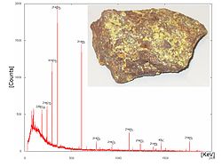Gamma-ray energy spectrum of ²³⁸U (inset). Gamma-rays are emitted by decaying nuclides, and the gamma-ray energy can be used to characterize the decay (which nuclide is decaying to which). Here, using the gamma-ray spectrum, several nuclides that are typical of the decay chain have been identified: ²²⁶Ra, ²¹⁴Pb, ²¹⁴Bi.

An example is the natural decay chain of ²³⁸U, which is as follows:

• decays, through alpha-emission, with a half-life of 4.5 billion years to thorium-234
• which decays, through beta-emission, with a half-life of 24 days to protactinium-234
• which decays, through beta-emission, with a half-life of 1.2 minutes to uranium-234
• which decays, through alpha-emission, with a half-life of 240 thousand years to thorium-230
• which decays, through alpha-emission, with a half-life of 77 thousand years to radium-226
• which decays, through alpha-emission, with a half-life of 1.6 thousand years to radon-222
• which decays, through alpha-emission, with a half-life of 3.8 days to polonium-218
• which decays, through alpha-emission, with a half-life of 3.1 minutes to lead-214
• which decays, through beta-emission, with a half-life of 27 minutes to bismuth-214
• which decays, through beta-emission, with a half-life of 20 minutes to polonium-214
• which decays, through alpha-emission, with a half-life of 160 microseconds to lead-210
• which decays, through beta-emission, with a half-life of 22 years to bismuth-210
• which decays, through beta-emission, with a half-life of 5 days to polonium-210
• which decays, through alpha-emission, with a half-life of 140 days to lead-206, which is a stable nuclide.

Some radionuclides may have several different paths of decay. For example, approximately 36% of bismuth-212 decays, through alpha-emission, to thallium-208 while approximately 64% of bismuth-212 decays, through beta-emission, to polonium-212. Both the thallium-208 and the polonium-212 are radioactive daughter products of bismuth-212, and both decay directly to stable lead-208.

Occurrence and applications

According to the Big Bang theory, stable isotopes of the lightest five elements (H, He, and traces of Li, Be, and B) were produced very shortly after the emergence of the universe, in a process called Big Bang nucleosynthesis. These lightest stable nuclides (including deuterium) survive to today, but any radioactive isotopes of the light elements produced in the Big Bang (such as tritium) have long since decayed. Isotopes of elements heavier than boron were not produced at all in the Big Bang, and these first five elements do not have any long-lived radioisotopes. Thus, all radioactive nuclei are, therefore, relatively young with respect to the birth of the universe, having formed later in various other types of nucleosynthesis in stars (in particular, supernovae), and also during ongoing interactions between stable isotopes and energetic particles. For example, carbon-14, a radioactive nuclide with a half-life of only 5730 years, is constantly produced in Earth's upper atmosphere due to interactions between cosmic rays and nitrogen.

Radioactive decay has been put to use in the technique of radioisotopic labeling, which is used to track the passage of a chemical substance through a complex system (such as a living organism). A sample of the substance is synthesized with a high concentration of unstable atoms. The presence of the substance in one or another part of the system is determined by detecting the locations of decay events.

On the premise that radioactive decay is truly random (rather than merely chaotic), it has been used in hardware random-number generators. Because the process is not thought to vary significantly in mechanism over time, it is also a valuable tool in estimating the absolute ages of certain materials. For geological materials, the radioisotopes and some of their decay products become trapped when a rock solidifies, and can then later be used (subject to many well-known qualifications) to estimate the date of the solidification. These include checking the results of several simultaneous processes and their products against each other, within the same sample. In a similar fashion, and also subject to qualification, the rate of formation of carbon-14 in various eras, the date of formation of organic matter within a certain period related to the isotope's half-life may be estimated, because the carbon-14 becomes trapped when the organic matter grows and incorporates the new carbon-14 from the air. Thereafter, the amount of carbon-14 in organic matter decreases according to decay processes that may also be independently cross-checked by other means (such as checking the carbon-14 in individual tree rings, for example).

Radioactive decay rates

The decay rate, or activity, of a radioactive substance are characterized by:

Constant quantities:

• half-life — symbol t_1/2 — the time taken for the activity of a given amount of a radioactive substance to decay to half of its initial value.
• mean lifetime — symbol τ — the average lifetime of a radioactive particle before decay.
• decay constant — symbol λ — the inverse of the mean lifetime.

Although these are constants, they are associated with statistically random behavior of populations of atoms. In consequence predictions using these constants are less accurate for small number of atoms.

In principle a third-life, tenth-life, or even (1/√2)-life (the reciprocal of any real number greater than and not equal to 1) etc can of course be used in exactly the same way as half-life. The half-life is adopted as the standard time associated with exponential decay.

Time-variable quantities:

• Total activity — symbol A — number of decays per unit time of a radioactive sample.
• Number of particles — symbol N — the total number of particles in the sample.
• Specific activity — symbol S_A — number of decays per unit time per amount of substance of the sample at time set to zero (t = 0). "Amount of substance" can be the mass, volume or moles of the initial sample.

These are related as follows:

$t_{1/2} = \frac{\ln(2)}{\lambda} = \tau \ln(2)$

$A = - \frac{\mathrm{d}N}{\mathrm{d}t} = \lambda N$

$S_A a_0 = - \frac{\mathrm{d}N}{\mathrm{d}t}\bigg|_{t=0} = \lambda N_0$

where a₀ is the initial amount of active substance — substance that has the same percentage of unstable particles as when the substance was formed.

Activity measurements

The units in which activities are measured are: becquerel (symbol Bq) = one disintegration per second; curie (Ci) = 3.7 × 10¹⁰ Bq. Low activities are also measured in disintegrations per minute (dpm).

Mathematics of radioactive decay

For the mathematical details of exponential decay in general context, see exponential decay .

For the analogous mathematics in 1st order chemical reactions, see Consecutive reactions.

Universal law of radioactive decay

Radioactivity is one very frequent example of exponential decay. The law however is only statistical - not exact. In the following formalism, the number of nuclides or nuclide population N, is of course a descrete variable (a natural number) - but for any physical sample N is so large (amounts of L = 10^23, avagadro's constant) that it can be treated as a continuous variable. Differential calculus to set up differential equations for modelling the behaviour of the nuclear decay.

One-decay process

Consider the case of a nuclide A decaying into another B by some process, i.e. A → B (emission of other particles, like electron neutrinos ν
e and electrons e^– in beta decay, are irrelevant in what follows). The decay of an unstable nucleus is entirely random and it is impossible to predict when a particular atom will decay.^[1] However, it is equally likely to decay at any time. Therefore, given a sample of a particular radioisotope, the number of decay events (– dN) expected to occur in a small interval of time dt is proportional to the number of atoms present N, that is

$-\frac{\mathrm{d}N}{\mathrm{d}t} \propto N.$

Particular radionuclides decay at different rates, so each has its own decay constant λ (lower Greek lambda). The probability of decay (−dN/N) is proportional to an increment of time, dt:

$-\frac{\mathrm{d}N}{N} = \lambda \mathrm{d}t$

The negative sign indicates that N decreases as time increases, as each decay event follows one after another. The solution to this first-order differential equation is the function:

$N(t) = N_0\,e^{-{\lambda}t} = N_0\,e^{-t/ \tau}, \,\!$

where N₀ is the value of N at the time set to zero (t = 0).

This equation is of particular interest; the behaviour of numerous important quantities can be found from it (see below). Although the parent decay distribution follows an exponential, observations of decay times will be limited by a finite integer number of N atoms and follow Poisson statistics as a consequence of the random nature of the process.

We have for all time t:

N_A + N_B = N_total = N_A0,

where N_total is the constant number of particles throughout the decay process, clearly equal to the initial number of A nuclides since this is the initial substance.

If the number of non-decayed A nuclei is:

$N_A = N_{A0}e^{-{\lambda}t} \,\!$

then the number of nuclei of B, i.e. number of decayed A nuclei, is

$N_B = N_{A0} - N_A = N_{A0} - N_{A0}e^{-{\lambda}t} = N_{A0} \left ( 1 - e^{-{\lambda}t} \right ).$

Chain-decay processes

Chain of two decays

Now consider the case of a chain of two decays: one nuclide A decaying into another B by one process, then B decaying into another C by a second process, i.e. A → B → C. The previous equation cannot be applied to a decay chain, but can be generalized as follows. The decay rate of B is proportional to the number of nuclides of B present, so again we have :

$-\frac{\mathrm{d}N_B}{\mathrm{d}t} \propto N_B,$

but care must be taken. Since A decays into B, then B decays into C, the activity of A adds to the total number of B nuclides in the present sample, before those B nuclides decay and reduce the number of nuclides leading to the later sample. In other words, the number of 2nd generation nuclei B increases as a result of the 1st generation nuclei decay of A, and decreases as a result of its own decay into the 3rd generation nuclei C ^[3]. The proportionality becomes an equation:

$\frac{\mathrm{d}N_B}{\mathrm{d}t} = - \lambda_B N_B,$

adding the increasing (and correcting) term obtains the law for a decay chain for two nuclides:

$\frac{\mathrm{d}N_B}{\mathrm{d}t} = -\lambda_B N_B + \lambda_A N_A.$

The equation is not

$\frac{\mathrm{d}N_B}{\mathrm{d}t} = - \left ( \lambda_B N_B + \lambda_A N_A \right ) ,$

since this implies the number of atoms of B is only decreasing as time increases, which is not the case. The rate of change of N_B, that is dN_B/dt, is related to the changes in the amounts of A and B, N_B can increase as B is produced from A and decrease as B produces C.

Re-writing using the previous results:

$\frac{\mathrm{d}N_B}{\mathrm{d}t} = - \lambda_B N_B + \lambda_A N_{A0} e^{-\lambda_A t}$

The subscripts simply refer to the respective nuclides, i.e. N_A is the number of nuclides of type A, N_A0 is the initial number of nuclides of type A, λ_A is the decay constant for A - and similarly for nuclide B. Solving this equation for N_B gives:

$N_B = \frac{N_{A0}\lambda_A}{\lambda_B - \lambda_A} \left ( e^{-\lambda_A t} - e^{-\lambda_B t}\right ) .$

Naturally this equation reduces to the previous solution, in the case B is a stable nuclide (λ_B = 0):

$\lim_{\lambda_B\rightarrow 0} \left [ \frac{N_{A0}\lambda_A}{\lambda_B - \lambda_A} \left ( e^{-\lambda_A t} - e^{-\lambda_B t}\right ) \right ] = \frac{N_{A0}\lambda_A}{0 - \lambda_A} \left ( e^{-\lambda_A t} - 1 \right ) = N_{A0} \left ( 1- e^{-\lambda_A t} \right ),$

as shown above for one decay. The solution can be found by the integration factor method, where the integrating factor is $e^{\lambda_B t}$. This case is perhaps the most useful, since it can derive both the one-decay equation (above) and the equation for multi-decay chains (below) more directly.

Chain of any number of decays

For the general case of any number of consecutive decays in a decay chain, i.e. A₁ → A₂ ... → A_i ... → A_D, where D is the number of decays and i is a dummy index (i = 1,2,3...D), each nuclide population can be found in terms of the previous population, using the above result in a recursive form:

$\frac{\mathrm{d}N_j}{\mathrm{d}t} = - \lambda_j N_j + \lambda_{j-1} N_{(j-1)0} e^{-\lambda_{j-1} t}.$

The general solution to the recursive problem are given by Bateman's equations ^[4]:

$\frac{\mathrm{d}N_D}{\mathrm{d}t} = N_0 \sum_{i=1}^D c_i e^{-\lambda_i t}$ $c_i = \frac{\prod_{j=1}^D \lambda_j}{\prod_{j=1, i\neq j}^D \left ( \lambda_j - \lambda_i \right )}$

Alternative decay modes

In all of the above examples, the initial nuclide decays into only one product. Consider the case of one initial nuclide which can decay into two products, that is A → B + C. We have for all time t:

N_A + N_B + N_C = N_total = N_A0,

in which,

$- \frac{\mathrm{d}N_A}{\mathrm{d}t} = \lambda_A N_A,$

$- \frac{\mathrm{d}N_B}{\mathrm{d}t} = \lambda_B N_A,$

$- \frac{\mathrm{d}N_C}{\mathrm{d}t} = \lambda_C N_A,$

so the relations follow in parallel:

$- \frac{\mathrm{d}N_A}{\mathrm{d}t} = - \frac{\mathrm{d}N_B}{\mathrm{d}t} - \frac{\mathrm{d}N_C}{\mathrm{d}t} = \lambda_A N_A = N_A \left ( \lambda_B + \lambda_C \right ) = N_A \lambda_A = \lambda_A \left [ N_{A0} - \left ( N_B + N_C \right ) \right ],$

indicating that the total decay constant is that of A, given by:

λ_A = λ_B + λ_C.

Solving this equation for N_A:

$N = N_{A0} e^{-\lambda_A t} .$

When measuring the production of one nuclide, one can only observe the total decay constant λ_A. The decay constants λ_B and λ_C determine the probability for the decay to result in products B or C as follows:

$N_B = \frac{\lambda_B}{\lambda_A} N_{A0} \left ( 1 - e^{-\lambda_A t} \right ),$

$N_C = \frac{\lambda_C}{\lambda_A} N_{A0} \left ( 1 - e^{-\lambda_A t} \right ).$

These perhaps seemingly disjionted results are consistent:

$\begin{align} N_B + N_C & = \frac{\lambda_B}{\lambda_A} N_{A0} \left ( 1 - e^{-\lambda_A t} \right ) + \frac{\lambda_C}{\lambda_A} N_{A0} \left ( 1 -e^{-\lambda_A t} \right ) \\ & = \left ( \frac{\lambda_B}{\lambda_B + \lambda_C} + \frac{\lambda_C}{\lambda_B + \lambda_C} \right ) N_{A0} \left ( 1 -e^{-\lambda_A t} \right ) = N_{A0} \left ( 1 -e^{-\lambda_A t} \right ) \\ & = N_{A0} - N_{A0} e^{-\lambda_A t} = N_\mathrm{total} - N_A . \end{align}$

Corollaries of the decay laws

The solutions to the above differential equations are sometimes written using quantities related to the number of nuclides, such as:

• the activity A of a sample relates to N by: $A = \lambda N , \,\!$
• the number of moles (aka amount of substance) n of sample relates to N via L = 6.023 × 10²³ (Avagadro's constant) by: $N = L n , \,\!$
• the mass M of the sample relates to N via relative atomic mass number A_r (or A_r) by: $M = A_r n = A_r N / L , \,\!$
• collecting these results together for conveinence: $N = \frac{A}{\lambda} = L n = \frac{LM}{A_r} .\,\!$

Equivalant ways to write the decay solutions are as follows:

One-decay processes

The solution

$N = N_0\,e^{-\lambda t} , \,\!$

can be written:

$A = A_0\,e^{-\lambda t} , \,\!$

$n = n_0\,e^{-\lambda t} , \,\!$

$M = M_0\,e^{-\lambda t} , \,\!$

Notice how we can simply replace each quantity (on both sides of the equation), since they are directly proportional to N and so the constants cancel (constant at least for a particular nuclide).

Chain-decay processes

For the two-decay chain,

$N_B = \frac{N_{A0}\lambda_A}{\lambda_B - \lambda_A} \left ( e^{-\lambda_A t} - e^{-\lambda_B t}\right ) ,$

its almost as simple:

$A_B = \frac{A_{A0}\lambda_B}{\lambda_B - \lambda_A} \left ( e^{-\lambda_A t} - e^{-\lambda_B t}\right ) ,$

$M_B = \frac{A_r \left ( \mathrm{B} \right ) M_{A0}\lambda_A}{ A_r \left ( \mathrm{A} \right ) \left ( \lambda_B - \lambda_A \right )} \left ( e^{-\lambda_A t} - e^{-\lambda_B t}\right ) ,$

$n_B = \frac{n_{A0}\lambda_A}{\lambda_B - \lambda_A} \left ( e^{-\lambda_A t} - e^{-\lambda_B t}\right ) .$

Decay timing: definitions and relations

Time constant and mean-life

For the one-decay solution (A → B):

$N = N_0\,e^{-{\lambda}t} = N_0\,e^{-t/ \tau}, \,\!$

the equation indicates that the decay constant λ has units of 1/time, and can thus also be represented as 1/τ, where τ is a characteristic time for the process: called the time constant of the process.

In radioactive decay, this process time constant is also the mean lifetime for decaying atoms. Each atom "lives" for a finite amount of time before it decays, and it may be shown that this mean lifetime is the arithmetic mean of all the atoms' lifetimes, and that it is τ, which again is related to the decay constant as follows:

$\tau = \frac{1}{\lambda}.$

This form is also true for two-decay processes simaltaneously (A → B + C), inserting the equivalent values of decay constants (as given above)

$\lambda = \lambda_B + \lambda_C \,$

into the decay solution leads to:

$\frac{1}{\tau} = \lambda = \lambda_B + \lambda_C = \frac{1}{\tau_B} + \frac{1}{\tau_C}\,$

Simulation of many identical atoms undergoing radioactive decay, starting with either 4 atoms (left) or 400 (right). The number at the top indicates how many half-lives have elapsed. Note the law of large numbers: with more atoms, the overall decay is less random.

Half-life

A more commonly used parameter is the half-life. Given a sample of a particular radionuclide, the half-life is the time taken for half the radionuclide's atoms to decay. For the case of one-decay nuclear reactions:

$N = N_0\,e^{-{\lambda}t} = N_0\,e^{-t/ \tau}, \,\!$

the half-life is related to the decay constant as follows: set N = N₀/2 and t = T_1/2 to obtain

$t_{1/2} = \frac{\ln 2}{\lambda} = \tau \ln 2.$

This relationship between the half-life and the decay constant shows that highly radioactive substances are quickly spent, while those that radiate weakly endure longer. Half-lives of known radionuclides vary widely, from more than 10¹⁹ years (such as for very nearly stable nuclides, e.g., ²⁰⁹Bi), to 10⁻²³ seconds for highly unstable ones.

The factor of ln2 in the above relations results from the fact that concept of "half-life" is merely a way of selecting a different base other than the natural base e for the lifetime expression. The time constant τ is the "1/e" life (time till only 1/e = about 36.8% remains) rather than the "1/2" life of a radionuclide where 50% remains (thus, τ is longer than t_½). Thus, the following equation can be shown to be equaly valid:

$N(t) = N_0\,e^{-t/ \tau} =N_0\,2^{-t/t_{1/2}}. \,\!$

Since radioactive decay is exponential with a constant probability, each process could as easily be described with a different constant time period that (for example) gave its "1/3-life" (how long until only 1/3 is left) or "1/10-life" (a time period till only 10% is left), and so on. Thus, the choice of τ and t_½ for marker-times, are only for convenience, and from convention. They reflect a fundamental principle only in so much as they show that the same proportion of a given radioactive substance will decay, during any time-period that one chooses.

Mathematically, the n-th life for the above situation would be found in the same way as above - by setting N = N₀/n, t = T_1/n and substituing into the deacy solution to obtain

$t_{1/n} = \frac{\ln n}{\lambda} = \tau \ln n.$

Example

A sample of ¹⁴C, whose half-life is 5730 years, has a decay rate of 14 disintegration per minute (dpm) per gram of natural carbon. An artefact is found to have radioactivity of 4 dpm per gram of its present C, how old is the artefact?

Using the above equation, we have:

$N = N_0\,e^{-t/ \tau},$

where: $\frac{N}{ N_0} = 4/14 \approx 0.286,$

$\tau = \frac{T_{1/2}}{\ln 2} \approx 8267$ years,

$t = -\tau\,\ln\frac{N}{ N_0} \approx 10360$ years.

Changing decay rates

The radioactive decay modes of electron capture and internal conversion are known to be slightly sensitive to chemical and environmental effects which change the electronic structure of the atom, which in turn affects the presence of 1s and 2s electrons that participate in the decay process. A small number of mostly light nuclides are affected. For example, chemical bonds can affect the rate of electron capture to a small degree (in general, less than 1%) depending on the proximity of electrons to the nucleus in beryllium. In ⁷Be, a difference of 0.9% has been observed between half-lives in metallic and insulating environments.^[5] This relatively large effect is because beryllium is a small atom whose valence electrons are in 2s atomic orbitals, which are subject to electron capture in ⁷Be because (like all s atomic orbitals in all atoms) they naturally penetrate into the nucleus.

Rhenium-187 is a more spectacular example. ¹⁸⁷Re normally beta decays to ¹⁸⁷Os with a half-life of 41.6 × 10⁹ y,^[6] but studies using fully ionised ¹⁸⁷Re atoms (bare nuclei) have found that this can decrease to only 33 y. This is attributed to "bound-state β^- decay" of the fully ionised atom — the electron is emitted into the "K-shell" (1s atomic orbital), which cannot occur for neutral atoms in which all low-lying bound states are occupied.^[7]

A number of experiments have found that decay rates of other modes of artificial and naturally-occurring radioisotopes are, to a high degree of precision, unaffected by external conditions such as temperature, pressure, the chemical environment, and electric, magnetic, or gravitational fields.^{[citation needed]} Comparison of laboratory experiments over the last century, studies of the Oklo natural nuclear reactor (which exemplified the effects of thermal neutrons on nuclear decay), and astrophysical observations of the luminosity decays of distant supernovae (which occurred far away so the light has taken a great deal of time to reach us), for example, strongly indicate that decay rates have been constant (at least to within the limitations of small experimental errors) as a function of time as well.

Recent results suggest the possibility that decay rates might have a weak dependence (0.5% or less) on environmental factors. It has been suggested that measurements of decay rates of silicon-32, manganese-54, and radium-226 exhibit small seasonal variations (of the order of 0.1%), proposed to be related to either solar flare activity or distance from the sun.^[8][9][10] However, such measurements are highly susceptible to systematic errors, and a subsequent paper^[11] has found no evidence for such correlations in six other isotopes, and sets upper limits on the size of any such effects.

See also

• Actinides in the environment
• Background radiation
• Chernobyl disaster
• Decay chain
• Fallout shelter
• Half-life
• Lists of nuclear disasters and radioactive incidents
• National Council on Radiation Protection and Measurements
• Nuclear medicine
• Nuclear pharmacy
• Nuclear physics
• Nuclear power
• Particle decay
• Poisson process
• Radiation
• Radiation therapy
• Radioactive contamination
• Radioactivity in biology
• Radiometric dating
• Radionuclide a.k.a. "radio-isotope"
• Secular equilibrium
• Transient equilibrium

Notes

1. ^ ^{a b} "Decay and Half Life". http://www.iem-inc.com/prhlfr.html. Retrieved 2009-12-14. 
2. ^ Hrabak, M. et al (July 2008). "Nikola Tesla and the Discovery of X-rays". RadioGraphics 28 (4): 1189–92. doi:10.1148/rg.284075206. PMID 18635636. 
3. ^ Introductory Nuclear Physics, K.S. Krane, 1988, John Wiley & Sons Inc, ISBN978-0-471-80553-3
4. ^ Introductory Nuclear Physics, K.S. Krane, 1988, John Wiley & Sons Inc, ISBN978-0-471-80553-3
5. ^ B.Wang et al., Euro. Phys. J. A 28, 375-377 (2006) Change of the ⁷Be electron capture half-life in metallic environments
6. ^ Smoliar, M.I.; Walker, R.J.; Morgan, J.W. (1996). "Re-Os ages of group IIA, IIIA, IVA, and IVB iron meteorites". Science 271 (5252): 1099–1102. Bibcode 1996Sci...271.1099S. doi:10.1126/science.271.5252.1099. 
7. ^ Bosch, F.; Faestermann, T.; Friese, J.; Heine, F.; Kienle, P.; Wefers, E.; Zeitelhack, K.; Beckert, K. et al. (1996). "Observation of bound-state β– decay of fully ionized ¹⁸⁷Re:¹⁸⁷Re-¹⁸⁷Os Cosmochronometry". Physical Review Letters 77 (26): 5190–5193. Bibcode 1996PhRvL..77.5190B. doi:10.1103/PhysRevLett.77.5190. PMID 10062738. 
8. ^ "The mystery of varying nuclear decay". Physics World. October 2, 2008. http://physicsworld.com/cws/article/news/36108. 
9. ^ "Perturbation of Nuclear Decay Rates During the Solar Flare of 13 December 2006". Astroparticle Physics 31 (6): 407–411. 2009. arXiv:0808.3156. Bibcode 2009APh....31..407J. doi:10.1016/j.astropartphys.2009.04.005. 
10. ^ Jenkins, J. H.; et al. (2009). "Evidence of correlations between nuclear decay rates and Earth–Sun distance". Astroparticle Physics 32 (1): 42–46. arXiv:0808.3283. Bibcode 2009APh....32...42J. doi:10.1016/j.astropartphys.2009.05.004. 
11. ^ Norman, E. B.; et al. (2009). "Evidence against correlations between nuclear decay rates and Earth–Sun distance". Astroparticle Physics 31 (2): 135–137. Bibcode 2009APh....31..135N. doi:10.1016/j.astropartphys.2008.12.004. http://donuts.berkeley.edu/papers/EarthSun.pdf. 

References

• "Radioactivity", Encyclopædia Britannica. 2006. Encyclopædia Britannica Online. December 18, 2006
• Radio-activity by Ernest Rutherford Phd, Encyclopædia Britannica Eleventh Edition

External links

• The Lund/LBNL Nuclear Data Search – Contains tabulated information on radioactive decay types and energies.
• NUCLEONICA Nuclear Science Portal
• NUCLEONICA wiki: Decay Engine
• Nomenclature of nuclear chemistry
• Some theoretical questions of nuclear stability
• Specific activity and related topics.
• The Karlsruhe Nuclide Chart
• Monte Carlo Simulation of Radioactive Decay
• The Live Chart of Nuclides – IAEA in Java or HTML
• Health Physics Society Public Education Website
•  "Becquerel Rays". The New Student's Reference Work. Chicago: F. E. Compton and Co. 1914. 
• Annotated bibliography for radioactivity from the Alsos Digital Library for Nuclear Issues
• Stochastic Java applet on the decay of radioactive atoms by Wolfgang Bauer
• Stochastic Flash simulation on the decay of radioactive atoms by David M. Harrison