Voronoi diagram

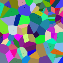The Voronoi diagram of a random set of points in the plane (all points lie within the image).

In mathematics, a Voronoi diagram is a special kind of decomposition of a given space, e.g., a metric space, determined by distances to a specified family of objects (subsets) in the space. These objects are usually called the sites or the generators (but other names such as "seeds" are in use) and to each such an object one associates a corresponding Voronoi cell, namely the set of all points in the given space whose distance to the given object is not greater than their distance to the other objects. It is named after Georgy Voronoi, and is also called a Voronoi tessellation, a Voronoi decomposition, or a Dirichlet tessellation (after Lejeune Dirichlet). Voronoi diagrams can be found in a large number of fields in science and technology, even in art, and they have found numerous practical and theoretical applications.^[1][2]

The simplest case

In the simplest and most familiar case (shown in the first picture), we are given a finite set of points {p₁,...,p_n} in the Euclidean plane. In this case each site p_k is simply a point, and its corresponding Voronoi cell (also called Voronoi region or Dirichlet cell) R_k consisting of all points whose distance to p_k is not greater than their distance to any other site. Each such cell is obtained from the intersection of half-spaces, and hence it is a convex polygon. The segments of the Voronoi diagram are all the points in the plane that are equidistant to the two nearest sites. The Voronoi vertices (nodes) are the points equidistant to three (or more) sites.

Formal definition

Let X be a space (a nonempty set) endowed with a distance function d. Let K be a set of indices and let (P_k)_{k ∈ K} be a tuple (ordered collection) of nonempty subsets (the sites) in the space X. The Voronoi cell, or Voronoi region, R_k, associated with the site P_k is the set of all points in X whose distance to P_k is not greater than their distance to the other sites P_j , where j is any index different from k. In other words, if d(x,A)=inf{d(x,a): a in A} denotes the distance between the point x and the subset A, then

R_k={x in X: d(x,P_k) ≤ d(x,P_j) for all j≠k}.

The Voronoi diagram is simply the tuple of cells (R_k)_{k ∈ K} . In principle some of the sites can intersect and even coincide (an application is described below for sites representing shops), but usually they are assumed to be disjoint. In addition, infinitely many sites are allowed in the definition (this setting has applications in geometry of numbers and crystallography), but again, in many cases only finitely many sites are considered.

In the particular case where the space is a finite dimensional Euclidean space, each site is a point, there are finitely many points and all of them are different, then the Voronoi cells are convex polytopes and they can be represented in a combinatorial way using their vertices, sides, 2-dimensional faces, etc. Sometimes the induced combinatorial structure is referred to as the Voronoi diagram. However, in general the Voronoi cells may not be convex or even connected.

Illustration

As a simple illustration, consider a group of shops in a flat city. Suppose we want to estimate the number of customers of a given shop. With all else being equal (price, products, quality of service, etc.), it is reasonable to assume that customers choose their preferred shop simply by distance considerations: they will go to the shop located nearest to them. In this case the Voronoi cell R_k of a given shop P_k can be used for giving a rough estimate on the number of potential customers going to this shop (which is modeled by point in our flat city).

So far it was assumed that the distance between points in the city are measured using the standard distance, namely the Euclidean distance: d((a₁,a₂),(b₁,b₂))=((a₁-b₁)²+(a₂-b₂)²)^0.5. However, if we consider the case where customers only go to the shops by a vehicle and the traffic paths are parallel to the x and y axes, like in Manhattan, then a more realistic distance function will be the l₁ distance, namely d((a₁,a₂),(b₁,b₂))=|a₁-b₁|+|a₂-b₂|.

Properties

• The dual graph for a Voronoi diagram (in the case of a Euclidean space with point sites) corresponds to the Delaunay triangulation for the same set of points.
• The closest pair of points corresponds to two adjacent cells in the Voronoi diagram.
• Assume the setting is the Euclidean plane and a group of different points are given. Then two points are adjacent on the convex hull if and only if their Voronoi cells share an infinitely long side.
• If the space is a normed space and the distance to each site is attained (e.g., when a site is a compact set or a closed ball), then each Voronoi cell can be represented as a union of line segments emanating from the sites ^[3]. As shown there, this property does not necessarily hold when the distance is not attained.
• Under relatively general conditions (the space is a possibly infinite dimensional uniformly convex space, there can be infinitely many sites of a general form, etc.) Voronoi cells enjoy a certain stability property: a small change in the shapes of the sites, e.g., a change caused by some translation or distortion, yields a small change in the shape of the Voronoi cells. This is the geometric stability of Voronoi diagrams ^[4]. As shown there, this property does not hold in general, even if the space is two-dimensional (but non-uniformly convex, and, in particular, non-Euclidean) and the sites are points.

History

Informal use of Voronoi diagrams can be traced back to Descartes in 1644. Dirichlet used 2-dimensional and 3-dimensional Voronoi diagrams in his study of quadratic forms in 1850. British physician John Snow used a Voronoi diagram in 1854 to illustrate how the majority of people who died in the Soho cholera epidemic lived closer to the infected Broad Street pump than to any other water pump.

Voronoi diagrams are named after Russian mathematician Georgy Fedoseevich Voronoi (or Voronoy) who defined and studied the general n-dimensional case in 1908. Voronoi diagrams that are used in geophysics and meteorology to analyse spatially distributed data (such as rainfall measurements) are called Thiessen polygons after American meteorologist Alfred H. Thiessen. In condensed matter physics, such tessellations are also known as Wigner-Seitz unit cells. Voronoi tessellations of the reciprocal lattice of momenta are called Brillouin zones. For general lattices in Lie groups, the cells are simply called fundamental domains. In the case of general metric spaces, the cells are often called metric fundamental polygons.

Examples

This is a slice of the Voronoi diagram of a random set of points in a 3D box. In general a cross section of a 3D Voronoi tessellation is not a 2D Voronoi tessellation itself. (The cells are all convex polyhedra.)

Voronoi tessellations of regular lattices of points in two or three dimensions give rise to many familiar tessellations.

• A 2D lattice gives an irregular honeycomb tessellation, with equal hexagons with point symmetry; in the case of a regular triangular lattice it is regular; in the case of a rectangular lattice the hexagons reduce to rectangles in rows and columns; a square lattice gives the regular tessellation of squares; note that the rectangles and the squares can also be generated by other lattices (for example the lattice defined by the vectors (1,0) and (1/2,1/2) gives squares). See here for a dynamic visual example.
• A simple cubic lattice gives the cubic honeycomb.
• A hexagonal close-packed lattice gives a tesselation of space with trapezo-rhombic dodecahedra.
• A face-centred cubic lattice gives a tessellation of space with rhombic dodecahedra.
• A body-centred cubic lattice gives a tessellation of space with truncated octahedra.
• Parallel planes with regular triangular lattices aligned with each others' centers give the hexagonal prismatic honeycomb.
• Certain body centered tetragonal lattices give a tessellation of space with rhombo-hexagonal dodecahedra.

For the set of points (x, y) with x in a discrete set X and y in a discrete set Y, we get rectangular tiles with the points not necessarily at their centers.

Higher-order Voronoi diagrams

Although a normal Voronoi cell is defined as the set of points closest to a single point in S, an nth-order Voronoi cell is defined as the set of points having a particular set of n points in S as its n nearest neighbors. Higher-order Voronoi diagrams also subdivide space.

Higher-order Voronoi diagrams can be generated recursively. To generate the n^th-order Voronoi diagram from set S, start with the (n − 1)^th-order diagram and replace each cell generated by X = {x₁, x₂, ..., x_n−1} with a Voronoi diagram generated on the set S − X.

Farthest-Point Voronoi Diagram

For a set of n points the (n−1)^th-order Voronoi diagram is called a Farthest-Point Voronoi diagram.

For a given set of points S = {p₁, p₂, ..., p_n} the Farthest-Point Voronoi Diagram divides the plane into cells in which the same point of P is the farthest point. Note that a point of P has a cell in the Farthest-Point Voronoi diagram if and only if it is a vertex of the convex hull of P. Thus, let H = {h₁, h₂, ..., h_k} be the convex hull of P we define the Farthest-Point Voronoi diagram as the subdivision of the plane into k cells, one for each point in H, with the property that a point q lies in the cell corresponding to a site h_i if and only if dist(q, h_i) > dist(q, p_j) for each p_j∈S with h_i ≠ p_j. Where dist(p, q) is the euclidean distance between two points p and q.^{[5] [6]}

Generalizations and variations

As implied by the definition, Voronoi cells can be defined for metrics other than Euclidean (such as the Mahalanobis or Manhattan) distances. However in these cases the boundaries of the Voronoi cells may be more complicated than in the Euclidean case, since the equidistant locus for two points may fail to be subspace of codimension 1, even in the 2-dimensional case.

A weighted Voronoi diagram is the one in which the function of a pair of points to define a Voronoi cell is a distance function modified by multiplicative or additive weights assigned to generator points. In contrast to the case of Voronoi cells defined using a distance which is a metric, in this case some of the Voronoi cells may be empty.

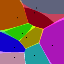Approximate Voronoi diagram of a set of points. Notice the blended colors in the fuzzy boundary of the Voronoi cells.

The Voronoi diagram of n points in d-dimensional space requires $O(n^{\lceil d/2 \rceil})$ storage space. Therefore, Voronoi diagrams are often not feasible for d > 2. An alternative is to use approximate Voronoi diagrams, where the Voronoi cells have a fuzzy boundary, which can be approximated.^[7]

Voronoi diagram are also related to other geometric structures such as the medial axis (which has found applications in image segmentation, optical character recognition and other computational applications) and the straight skeleton.

Applications

• One of the early applications of Voronoi diagrams was by John Snow to study the epidemiology of the 1854 Broad Street cholera outbreak in Soho, England. He showed the correlation between areas on the map of London using a particular water pump, and the areas with most deaths due to the outbreak.

• A point location data structure can be built on top of the Voronoi diagram in order to answer nearest neighbor queries, where one wants to find the object that is closest to a given query point. Nearest neighbor queries have numerous applications. For example, one might want to find the nearest hospital, or the most similar object in a database. A large application is vector quantization, commonly used in data compression.

• With a given Voronoi diagram, one can also find the largest empty circle amongst a set of points, and in an enclosing polygon; e.g. to build a new supermarket as far as possible from all the existing ones, lying in a certain city.

• Voronoi diagrams together with Farthest-Point Voronoi diagrams are used for efficient algorithms to compute the roundness of a set of points.^[5]

• The Voronoi diagram is useful in polymer physics. It can be used to represent free volume of the polymer.

• It is also used in derivations of the capacity of a wireless network.

• In climatology, Voronoi diagrams are used to calculate the rainfall of an area, based on a series of point measurements. In this usage, they are generally referred to as Thiessen polygons.

• Voronoi diagrams are used to study the growth patterns of forests and forest canopies, and may also be helpful in developing predictive models for forest fires.

• Voronoi diagrams are also used in computer graphics to procedurally generate some kinds of organic looking textures.

• In autonomous robot navigation, Voronoi diagrams are used to find clear routes. If the points are obstacles, then the edges of the graph will be the routes furthest from obstacles (and theoretically any collisions).

• In computational chemistry, Voronoi cells defined by the positions of the nuclei in a molecule are used to compute atomic charges. This is done using the Voronoi deformation density method.

• In materials science, polycrystalline microstructures in metallic alloys are commonly represented using Voronoi tessellations.

• Voronoi Polygons have been used in mining to estimate the reserves of valuable materials, minerals or other resources. Exploratory drillholes are used as the set of points in the Voronoi polygons.

See also

Algorithms

• Bowyer–Watson algorithm -- an algorithm for generating a Voronoi diagram in any number of dimensions.
• Fortune's algorithm -- an O(n log(n)) algorithm for generating a Voronoi diagram from a set of points in a plane.
• Lloyd's algorithm

Related subjects

• Centroidal Voronoi tessellation
• Computational geometry
• Delaunay triangulation
• Mathematical diagram
• Nearest neighbor search
• Nearest-neighbor interpolation
• Pole

Notes

1. ^ Franz Aurenhammer (1991). Voronoi Diagrams - A Survey of a Fundamental Geometric Data Structure. ACM Computing Surveys, 23(3):345-405, 1991
2. ^ Atsuyuki Okabe, Barry Boots, Kokichi Sugihara & Sung Nok Chiu (2000). Spatial Tessellations - Concepts and Applications of Voronoi Diagrams. 2nd edition. John Wiley, 2000, 671 pages ISBN 0-471-98635-6
3. ^ Daniel Reem, An algorithm for computing Voronoi diagrams of general generators in general normed spaces, In Proceedings of the sixth International Symposium on Voronoi Diagrams in science and engineering (ISVD 2009), 2009, pp. 144--152
4. ^ Daniel Reem, The geometric stability of Voronoi diagrams with respect to small changes of the sites, Full version: arXiv 1103.4125 (2011), Extended abstract in Proceedings of the 27th Annual ACM Symposium on Computational Geometry (SoCG ‏2011), pp. 254-263
5. ^ ^{a b} Mark de Berg, Marc van Kreveld, Mark Overmars, and Otfried Schwarzkopf (2008). Computational Geometry (Third edition ed.). Springer-Verlag.  7.4 Farthest-Point Voronoi Diagrams. Includes a description of the algorithm.
6. ^ Skyum, Sven (1991). "A simple algorithm for computing the smallest enclosing circle". Information Processing Letters 37(1991)121-125. , Contains a simple algorithm to compute the Farthest-Point Voronoi Diagram.
7. ^ S. Arya, T. Malamatos, and D. M. Mount, Space-Efficient Approximate Voronoi Diagrams, Proc. 34th ACM Symp. on Theory of Computing (STOC 2002), pp. 721–730.

References

• Gustav Lejeune Dirichlet (1850). Über die Reduktion der positiven quadratischen Formen mit drei unbestimmten ganzen Zahlen. Journal für die Reine und Angewandte Mathematik, 40:209-227.
• "Nouvelles applications des paramètres continus à la théorie des formes quadratiques". Journal für die Reine und Angewandte Mathematik 133: 97–178. 1908. doi:10.1515/crll.1908.133.97. 
• Atsuyuki Okabe, Barry Boots, Kokichi Sugihara & Sung Nok Chiu (2000). Spatial Tessellations - Concepts and Applications of Voronoi Diagrams. 2nd edition. John Wiley, 2000, 671 pages ISBN 0-471-98635-6
• Aurenhammer, Franz (1991). "Voronoi Diagrams - A Survey of a Fundamental Geometric Data Structure". ACM Computing Surveys 23 (3): 345–405. doi:10.1145/116873.116880. 
• Bowyer, Adrian (1981). "Computing Dirichlet tessellations". The Computer Journal 24 (2): pp. 162-166. doi:10.1093/comjnl/24.2.162. 
• Reem, Daniel (2009). "An algorithm for computing Voronoi diagrams of general generators in general normed spaces". Proceedings of the sixth International Symposium on Voronoi Diagrams in science and engineering (ISVD 2009): pp. 144—152. doi:10.1109/ISVD.2009.23. 
• Daniel Reem (2011). The geometric stability of Voronoi diagrams with respect to small changes of the sites. Full version: arXiv 1103.4125 (2011), Extended abstract: in Proceedings of the 27th Annual ACM Symposium on Computational Geometry (SoCG ‏2011), pp. 254-263.
• Watson, David F. (1981). "Computing the n-dimensional tessellation with application to Voronoi polytopes". The Computer Journal 24 (2): 167–172. doi:10.1093/comjnl/24.2.167. 
• Mark de Berg, Marc van Kreveld, Mark Overmars, and Otfried Schwarzkopf (2000). Computational Geometry (2nd revised edition ed.). Springer-Verlag. ISBN 3-540-65620-0.  Chapter 7: Voronoi Diagrams: pp. 147–163. Includes a description of Fortune's algorithm.
• Rolf Klein (1989). Abstract voronoi diagrams and their applications. Lecture Notes in Computer Science. 333. Springer-Verlag. pp. 148—157. doi:10.1007/3-540-50335-8_31. ISBN 3540520554. 

External links

• Real time interactive Voronoi / Delaunay diagrams with draggable points, Java 1.0.2, 1996-1997
• Real time interactive Voronoi and Delaunay diagrams with source code
• Demo for various metrics
• Mathworld on Voronoi diagrams
• Qhull for computing the Voronoi diagram in 2-d, 3-d, etc.
• Voronoi Diagrams: Applications from Archaeology to Zoology
• Voronoi Diagrams in CGAL, the Computational Geometry Algorithms Library
• Voronoi Web Site : using Voronoi diagrams for spatial analysis
• More discussions and picture gallery on centroidal Voronoi tessellations
• Voronoi Diagrams by Ed Pegg, Jr., Jeff Bryant, and Theodore Gray, Wolfram Demonstrations Project.
• Nice explanation of voronoi diagram and visual implementation of fortune's algorithm