Orbital perturbation analysis (spacecraft)

Isaac Newton in his Philosophiæ Naturalis Principia Mathematica demonstrated that the gravitational force between two mass points is inversely proportional to the square of the distance between the points and fully solved corresponding "two-body problem" demonstrating that radius vector between the two points would describe an ellipse. But already for the three body problem no exact closed form analytical form could be found. Instead approximate methods were developed, this is the method of "Orbital perturbation analysis". With this technique a quite accurate mathematical description of the trajectories of all the planets could be obtained. Especially critical was the mathematical modeling of the orbit of the Moon as the deviations from a pure Kepler orbit around the Earth due to the gravitational force of the Sun (i.e. one has indeed the three body problem) are much larger than deviations of the orbits of the planets from Sun-centered Kepler orbits caused by the gravitational attraction between the planets. With the availability of digital computers and the easiness to propagate orbits with numerical methods this problem partly disappeared, the motion of all celestial bodies including planets, satellites, asteroids and comets can be modeled and predicted with almost perfect accuracy using the method of the numerical propagation of the trajectories. Never-the-less several analytical closed form expressions for the effect of such additional "perturbing forces" are still very useful

Orbital perturbation of spacecraft orbits

All celestial bodies of the Solar System follow in first approximation a Kepler orbit around a central body. For a satellite (artificial or natural) this central body is a planet. But both due to gravitational forces caused by the Sun and other celestial bodies and due to the flattening of its planet (caused by its rotation which makes the planet slightly oblate and therefore the result of the Shell theorem not fully applicable) the satellite will follow an orbit that deviates more from a pure Kepler orbit then what is the case for the planets.

The precise modeling of the motion of the Moon has because of this been a difficult task. The best and most accurate modeling for the Moon orbit before the availability of digital computers was obtained with the complicated Delunay and Brown's lunar theories.

But the most important of these perturbation effects, the precession of the orbital plane caused by the slightly oblate shape of the Earth, was already fully understood by Isaac Newton who estimated the oblateness of the Earth from the observed rate of precession of the orbital plane of the Moon.

For man-made spacecraft orbiting the Earth at comparatively low altitudes the deviations from a Kepler orbit are much larger than for the Moon. The approximation of the gravitational force of the Earth to be that of a homogeneous sphere gets worse the closer one gets to the Earth surface and the majority of the artificial Earth satellites are in orbits that are only a few hundred kilometers over the Earth surface. Further more they are (as opposed to the Moon) significantly affected by the solar radiation pressure because of their large cross-section to mass ratio, this applies in particular to 3-axis stabilized spacecraft with large solar arrays. In addition they are significantly affected by rarefied air unless above 800–1000 km (The air drag at high altitudes strongly depending on the solar activity!)

Mathematical approach

Consider any function

$g(x_1,x_2,x_3,v_1,v_2,v_3)\,$

of the position

$x_1,x_2,x_3\,$

and the velocity

$v_1,v_2,v_3\,$

From the chain rule of differentiation one gets that the time derivative of g is

$\dot{g}\ =\ \frac{\partial g }{\partial x_1}\ v_1\ + \ \frac{\partial g }{\partial x_2}\ v_2\ + \frac{\partial g }{\partial x_3}\ v_3\ + \ \frac{\partial g }{\partial v_1}\ f_1\ + \ \frac{\partial g }{\partial v_2}\ f_2\ + \ \frac{\partial g }{\partial v_3}\ f_3$

where $f_1\ ,\ f_2\ ,\ f_3$ are the components of the force per unit mass acting on the body.

If now g is a "constant of motion" for a Kepler orbit like for example an orbital element and the force is corresponding "Kepler force"

$(f_1\ ,\ f_2\ ,\ f_3)\ = \ - \frac {\mu} {r^3}\ (x_1\ ,\ x_2\ ,\ x_3)$

one has that $\dot{g}\ =\ 0\,$.

If the force is the sum of the "Kepler force" and an additional force (force per unit mass)

$(h_1\ ,\ h_2\ ,\ h_3)$

i.e.

$(f_1\ ,\ f_2\ ,\ f_3)\ = \ - \frac {\mu} {r^3}\ (x_1\ ,\ x_2\ ,\ x_3)\ +\ (h_1\ ,\ h_2\ ,\ h_3)$

one therefore has

$\dot{g}\ =\frac{\partial g }{\partial v_1}\ h_1\ + \ \frac{\partial g }{\partial v_2}\ h_2\ + \ \frac{\partial g }{\partial v_3}\ h_3$

and that the change of $g\,$ in the time from $t=t_1\,$ to $t=t_2\,$ is

$\Delta g\ =\ \int\limits_{t_1}^{t_2}\left(\frac{\partial g }{\partial v_1}\ h_1\ + \ \frac{\partial g }{\partial v_2}\ h_2\ + \ \frac{\partial g }{\partial v_3}\ h_3 \right)dt$

If now the additional force $(h_1\ ,\ h_2\ ,\ h_3)\,$ is sufficiently small that the motion will be close to that of a Kepler orbit one gets an approximate value for $\Delta g\,$ by evaluating this integral assuming $x_1(t),x_2(t),x_3(t)\,$ to precisely follow this Kepler orbit.

In general one wants to find an approximate expression for the change $\Delta g\,$ over one orbital revolution using the true anomaly $\theta\,$ as integration variable, i.e. as

$\Delta g\ =\ \int\limits_{0}^{2\pi}\left(\frac{\partial g }{\partial v_1}\ h_1\ + \ \frac{\partial g }{\partial v_2}\ h_2\ + \ \frac{\partial g }{\partial v_3}\ h_3 \right)\frac{r^2}{\sqrt{\mu p}}d\theta$

(1)

This integral is evaluated setting $r(\theta)=\frac {p}{1+e\cos \theta}\,$, the elliptical Kepler orbit in polar angles. For the transformation of integration variable from time to true anomaly it was used that the angular momentum $H\ =\ r^2\ \dot{\theta}\ =\ \sqrt{\mu p} \,$ by definition of the parameter $p\,$ for a Kepler orbit (see equation (13) of the Kepler orbit article).

For the very important case that the Kepler orbit is circular or almost circular

$r\ =\ p$ and (1) takes the simpler form

$\Delta g\ =\ \frac{P}{2\pi}\ \int\limits_{0}^{2\pi}\left(\frac{\partial g }{\partial v_1}\ h_1\ + \ \frac{\partial g }{\partial v_2}\ h_2\ + \ \frac{\partial g }{\partial v_3}\ h_3 \right)d\theta$

(2)

where $P\ =\ 2\pi\ r\ \sqrt{\frac{r}{\mu}}\,$ is the orbital period

Perturbation of the semi-major axis/orbital period

For an elliptic Kepler orbit the sum of the kinetic and the potential energy

$g = \frac{V^2}{2}-\frac {\mu} {r}$

where $V\,$ is the orbital velocity

is a constant and equal to

$g\ =\ -\frac {\mu} {2 \cdot a}$ (Equation (44) of the Kepler orbit article)

If $\bar{h}\,$ is the perturbing force and $\bar{V}\,$is the velocity vector of the Kepler orbit the equation (1) takes the form:

$\Delta g\ =\ \int\limits_{0}^{2\pi}\bar{V} \bar{h}\frac{r^2}{\sqrt{\mu p}}d\theta$

(3)

and for a circular or almost circular orbit

$\Delta g\ =\ \frac{P}{2\pi}\ \int\limits_{0}^{2\pi} \bar{V} \bar{h}d\theta$

(4)

From the change $\Delta g\,$ of the parameter $g\,$ the new semi-major axis $a\,$ and the new period $P\ =\ 2\pi\ a\ \sqrt{\frac{a}{\mu}}\,$ are computed (relations (43) and (44) of the Kepler orbit article).

Perturbation of the orbital plane

Let $\hat{g}\,$ and $\hat{h}\,$ make up a rectangular coordinate system in the plane of the reference Kepler orbit. If $\omega\,$ is the argument of perigee relative the $\hat{g}\,$ and $\hat{h}\,$ coordinate system the true anomaly $\theta\,$ is given by $\theta=u-\omega\,$ and the approximate change $\Delta \hat{z}\,$ of the orbital pole $\hat{z}\,$ (defined as the unit vector in the direction of the angular momentum) is

$\Delta \hat{z}\ =\ \int\limits_{0}^{2\pi}\frac{f_z }{V_t} (\hat{g} \cos u + \hat{h} \sin u)\frac{r^2}{\sqrt{\mu p}}du \quad \times \ \hat{z} =\ \frac{1}{\mu p}\left[\hat{g}\int\limits_{0}^{2\pi}f_z r^3 \cos u \ du +\ \hat{h}\int\limits_{0}^{2\pi}f_z r^3 \sin u \ du \right]\quad \times \ \hat{z}$

(5)

where $f_z\,$ is the component of the perturbing force in the $\hat{z}\,$ direction, $V_t=\sqrt{\frac{\mu}{p}}\ (1+e\ \cos\theta)\,$ is the velocity component of the Kepler orbit orthogonal to radius vector and $r=\frac{p}{1+e\ \cos\theta}\,$ is the distance to the center of the Earth.

For a circular or almost circular orbit (5) simplifies to

$\Delta \hat{z}\ =\ \frac{r^2}{\mu}\left[\hat{g}\int\limits_{0}^{2\pi}f_z \cos u \ du +\ \hat{h}\int\limits_{0}^{2\pi}f_z \sin u \ du \right]\quad \times \ \hat{z}$

(6)

Example

In a circular orbit a low-force propulsion system (Ion thruster) generates a thrust (force per unit mass) of $F\ \hat{z}\,$ in the direction of the orbital pole in the half of the orbit for which $\sin u\,$ is positive and in the opposite direction in the other half. The resulting change of orbit pole after one orbital revolution of duration $P\ =\ 2\pi\ r\ \sqrt{\frac{r}{\mu}}\,$ is

$\Delta \hat{z}\ =\ \frac{r^2}{\mu}\left[\ 2\ F\int\limits_{0}^{\pi}\sin u \ du \right]\quad \hat{h}\times \hat{z} = \ \frac{r^2}{\mu}\ 4\ F\ \quad \hat{g}$

(7)

The average change rate $\frac{\Delta \hat{z}}{P}\,$ is therefore

$\frac{\Delta \hat{z}}{P} =\ \frac{2}{\pi}\ \frac{F}{V}\ \hat{g}$

(8)

where $V\ =\ \sqrt{\frac{\mu}{r}},$ is the orbital velocity in the circular Kepler orbit.

Perturbation of the eccentricity vector

Rather than applying (1) and (2) on the partial derivatives of the orbital elements eccentricity and argument of perigee directly one should apply these relations for the eccentricity vector. First of all the typical application is a near-circular orbit. But there are also mathematical advantages working with the partial derivatives of the components of this vector also for orbits with a significant eccentricity.

Equations (60), (55) and (52) of the Kepler orbit article say that the eccentricity vector is

$\bar{e}=\frac{(V_t-V_0) \cdot \hat{r} - V_r \cdot \hat{t}}{V_0}$

(9)

where

$V_0 = \sqrt{\frac{\mu}{p}}$

(10)

$p = \frac{{(r \cdot V_t)}^2}{\mu }$

(11)

from which follows that

$\frac{\partial\bar{e}}{\partial V_r} = -\frac {1}{V_0} \hat{t}$

(12)

$\frac{\partial\bar{e}}{\partial V_t} = \frac {1}{V_0} \left(2\ \hat{r}-\frac{V_r}{V_t}\ \hat{t}\right)$

(13)

where

$V_r = \sqrt{\frac {\mu}{p}} \cdot e \cdot \sin \theta$

(14)

$V_t = \sqrt{\frac {\mu}{p}} \cdot (1 + e \cdot \cos \theta)$

(15)

(Equations (18) and (19) of the Kepler orbit article)

The eccentricity vector is by definition always in the osculating orbital plane spanned by $\hat{r}$ and $\hat{t}$ and formally there is also a derivative

$\frac{\partial\bar{e}}{\partial V_z} = -\frac {V_r}{V_0}\ \frac{\partial\hat{t}}{\partial V_z}$

with

$\frac{\partial\hat{t}}{\partial V_z} = \frac {1}{V_t}\ \hat{z}$

corresponding to the rotation of the orbital plane

But in practice the in-plane change of the eccentricity vector is computed as

$\begin{align} \Delta \bar{e}\ = &\frac {1}{V_0}\ \int\limits_{0}^{2\pi}\left(-\hat{t}\ f_r\ + \ \left(2\ \hat{r}-\frac{V_r}{V_t}\ \hat{t}\right)\ f_t\right)\frac{r^2}{\sqrt{\mu p}}du\ = \\ &\frac {1}{\mu}\ \int\limits_{0}^{2\pi}\left(-\hat{t}\ f_r\ + \ \left(2\ \hat{r}-\frac{V_r}{V_t}\ \hat{t}\right)\ f_t\right) r^2 du \end{align}$

(16)

ignoring the out-of-plane force and the new eccentricity vector

$\bar{e} + \Delta \bar{e}$

is subsequently projected to the new orbital plane orthogonal to the new orbit normal

$\hat{z} + \Delta \hat{z}$

computed as described above.

Example

The Sun is in the orbital plane of a spacecraft in a circular orbit with radius $r\,$ and consequently with a constant orbital velocity $V_0\ =\ \sqrt{\frac{\mu}{r}}$ . If $\hat{k}\,$ and $\hat{l}\,$ make up a rectangular coordinate system in the orbital plane such that $\hat{k}\,$ points to the Sun and assuming that the solar radiation pressure force per unit mass $F\,$ is constant one gets that

$\hat{r}=\cos(u)\ \hat{k}\ +\ \sin(u)\ \hat{l}\,$

$\hat{t}=-\sin(u)\ \hat{k}\ +\ \cos(u)\ \hat{l}\,$

$F_r=-\cos(u)\ F\,$

$F_t= \sin(u)\ F\,$

where $u\,$ is the polar angle of $\hat{r}\,$ in the $\hat{k}\,$, $\hat{l}\,$ system. Applying (2) one gets that

$\begin{align} \Delta \hat{e}\ & =\ \frac{P}{2\pi}\ \frac {1}{V_0}\ \int\limits_{0}^{2\pi}\left( (-\sin(u)\ \hat{k}\ +\ \cos(u)\ \hat{l}) \ F\ \cos(u)\ + \ 2\ (\cos(u)\ \hat{k}\ +\ \sin(u)\ \hat{l})\ F\ \sin(u)\right)\ du \\ & = P\ \frac{3}{2}\ \frac {1}{V_0}\ \ F\ \hat{l} \end{align}$

(17)

This means the eccentricity vector will gradually increase in the direction $\hat{l}\,$ orthogonal to the Sun direction. This is true for any orbit with a small eccentricity, the direction of the small eccentricity vector does not matter. As $P\,$ is the orbital period this means that the average rate of this increase will be $\frac{3}{2}\ \frac {F}{V_0}\,$

The effect of the Earth flattening

Figure 1: The unit vectors $\hat{\phi}\ ,\ \hat{\lambda}\ ,\ \hat{r}$

In the article Geopotential model the modeling of the gravitational field as a sum of spherical harmonics is discussed. The by far dominating term is the "J2-term". This is a "zonal term" and corresponding force is therefore completely in a longitudinal plane with one component $F_r\ \hat{r}\,$ in the radial direction and one component $F_\lambda\ \hat{\lambda}\,$ with the unit vector $\hat{\lambda}\,$ orthogonal to the radial direction towards north. These directions $\hat{r}\,$ and $\hat{\lambda}\,$ are illustrated in Figure 1.

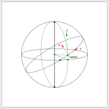Figure 2: The unit vector $\hat{t}\,$ orthogonal to $\hat{r}\,$ in the direction of motion and the orbital pole $\hat{z}\,$. The force component F_λ is marked as "F"

To be able to apply relations derived in the previous section the force component $F_\lambda\ \hat{\lambda}\,$ must be split into two orthogonal components $F_t\ \hat{t}$ and $F_z\ \hat{z}$ as illustrated in figure 2

Let $\hat{a}\ ,\ \hat{b}\ ,\ \hat{n}\,$ make up a rectangular coordinate system with origin in the center of the Earth (in the center of the Reference ellipsoid) such that $\hat{n}\,$ points in the direction north and such that $\hat{a}\ ,\ \hat{b}\,$ are in the equatorial plane of the Earth with $\hat{a}\,$ pointing towards the ascending node, i.e. towards the blue point of Figure 2.

The components of the unit vectors

$\hat{r}\ ,\ \hat{t}\ ,\ \hat{z}\,$

making up the local coordinate system (of which $\hat{t}\ ,\ \hat{z},$ are illustrated in figure 2) relative the $\hat{a}\ ,\ \hat{b}\ ,\ \hat{n}\,$ are

$r_a= \cos u\,$

$r_b= \cos i \ \sin u\,$

$r_n= \sin i \ \sin u\,$

$t_a=-\sin u\,$

$t_b= \cos i \ \cos u\,$

$t_n= \sin i \ \cos u\,$

$z_a= 0\,$

$z_b=-\sin i\,$

$z_n= \cos i\,$

where $u\,$ is the polar argument of $\hat{r}\,$ relative the orthogonal unit vectors $\hat{g}=\hat{a}\,$ and $\hat{h}=\cos i\ \hat{b}\ +\ \sin i\ \hat{n}\,$ in the orbital plane

Firstly

$\sin \lambda =\ r_n\ =\ \sin i \ \sin u\,$

where $\lambda\,$ is the angle between the equator plane and $\hat{r}\,$ (between the green points of figure 2) and from equation (12) of the article Geopotential model one therefore gets that

$f_r = J_2\ \frac{1}{r^4}\ \frac{3}{2}\ \left(3\ \sin^2 i\ \sin^2 u\ -\ 1\right)$

(18)

Secondly the projection of direction north, $\hat{n}\,$, on the plane spanned by $\hat{t}\ ,\ \hat{z},$ is

$\sin i \ \cos u \ \hat{t}\ +\ \cos i \ \hat{z}\,$

and this projection is

$\cos \lambda \ \hat{\lambda}\,$

where $\hat{\lambda}\,$ is the unit vector $\hat{\lambda}$ orthogonal to the radial direction towards north illustrated in figure 1.

From equation (12) of the article Geopotential model one therefore gets that

$f_\lambda \ \hat{\lambda}\ =\ -J_2\ \frac{1}{r^4}\ 3\ \sin\lambda\ (\sin i \ \cos u \ \hat{t}\ +\ \cos i \ \hat{z}) =\ -J_2\ \frac{1}{r^4}\ 3\ \sin i \ \sin u\ (\sin i \ \cos u \ \hat{t}\ +\ \cos i \ \hat{z})\,$

and therefore:

$f_t =\ -J_2\ \frac{1}{r^4}\ 3\ \sin^2 i\ \sin u\ \cos u$

(19)

$f_z =\ -J_2\ \frac{1}{r^4}\ 3\ \sin i\ \cos i\ \sin u$

(20)

Perturbation of the orbital plane

From (5) and (20) one gets that

$\Delta \hat{z}\ =\ -J_2\ \frac{3\ \sin i\ \cos i}{\mu p^2}\left[\hat{g}\int\limits_{0}^{2\pi}\frac{p}{r}\ \sin u\ \cos u \ du +\ \hat{h}\int\limits_{0}^{2\pi}\frac{p}{r}\ \sin^2 u\ du \right]\quad \times \ \hat{z}$

(21)

The fraction $\frac{p}{r}\,$ is

$\frac{p}{r}\ =\ 1\ +\ e\ \cos (u-\omega)\ =\ 1\ +\ e\ \cos u\ \cos\omega\ +\ e\ \sin u\ \sin\omega\,$

where $e\,$ is the eccentricity and $\omega\,$ is the argument of perigee of the reference Kepler orbit

As all integrals of type

$\int\limits_{0}^{2\pi} \cos^m u \ \sin^n u\ du\,$

are zero if not both $n\,$ and $m\,$ are even one gets from (21) that

$\Delta \hat{z}\ =\ -2\pi\ \frac{J_2}{\mu\ p^2}\ \frac{3}{2}\ \sin i\ \cos i\ \quad \hat{h} \times \hat{z}$

As

$\hat{n}\ =\ \cos i\ \hat{z}\ + \sin i\ \hat{h}$

this can be written

$\Delta \hat{z}\ =\ -2\pi\ \frac{J_2}{\mu\ p^2}\ \frac{3}{2}\ \cos i\ \quad \hat{n} \times \hat{z}$

(22)

As $\hat{n}$ is an inertially fixed vector (the direction of the spin axis of the Earth) relation (22) is the equation of motion for a unit vector $\hat{z}\,$ describing a cone around $\hat{n}$ with a precession rate (radians per orbit) of $-2\pi\ \frac{J_2}{\mu\ p^2}\ \frac{3}{2}\ \cos i\,$

In terms of orbital elements this is expressed as

$\Delta i\ =\ 0$

(23)

$\Delta \Omega\ =\ -2\pi\ \frac{J_2}{\mu\ p^2}\ \frac{3}{2}\ \cos i$

(24)

where

$i\,$ is the inclination of the orbit to the equatorial plane of the Earth

$\Omega\,$ is the right ascension of the ascending node

Perturbation of the eccentricity vector

From (16), (18) and (19) follows that in-plane perturbation of the eccentricity vector is

$\Delta \bar{e}\ =\ \frac {J_2}{\mu\ p^2}\ \int\limits_{0}^{2\pi}\left(-\hat{t}\ \left(\frac{p}{r}\right)^2\ \frac{3}{2}\ \left(3\ \sin^2 i\ \sin^2 u\ -\ 1\right)\ - \ \left(2\ \hat{r}-\frac{V_r}{V_t}\ \hat{t}\right)\ \left(\frac{p}{r}\right)^2\ 3\ \sin^2 i \cos u\ \sin u\right)du$

(25)

the new eccentricity vector being the projection of

$\bar{e}+\Delta \bar{e}$

on the new orbital plane orthogonal to

$\hat{z}+\Delta \hat{z}$

where $\Delta \hat{z}\,$ is given by (22)

Relative the coordinate system

$\hat{g}=\hat{a}\,$

$\hat{h}=\cos i\ \hat{b}\ +\ \sin i\ \hat{n}\,$

one has that

$\hat{r}=\cos u\ \hat{g}\ +\ \sin u\ \hat{h}\,$

$\hat{t}=-\sin u\ \hat{g}\ +\ \cos u\ \hat{h}\,$

Using that

$\frac {p}{r}\ =\ 1 + e \cdot \cos \theta\ =\ 1 + e_g \cdot \cos u + e_h \cdot \sin u$

and that

$\frac {V_r}{V_t} = \frac {e_g \cdot \sin u\ -\ e_h \cdot \cos u}{\frac {p}{r}}$

where

$e_g =\ e\ \cos \omega$

$e_h =\ e\ \sin \omega$

are the components of the eccentricity vector in the $\hat{g}\ ,\ \hat{h}\,$ coordinate system this integral (25) can be evaluated analytically, the result is

$\Delta \bar{e}\ =\ -2\pi\ \frac {J_2}{\mu\ p^2}\ \frac{3}{2} \left(\frac{3}{2}\ \sin^2 i\ -\ 1\right)\ \left(-e_h \hat{g}\ +\ e_g \hat{h}\right)\ =\ -2\pi\ \frac {J_2}{\mu\ p^2} \frac{3}{2} \left(\frac{3}{2}\ \sin^2 i\ -\ 1\right)\ \hat{z}\ \times \ \bar{e}$

(26)

This the difference equation of motion for the eccentricity vector $\bar{e}\,$ to form a circle, the magnitude of the eccentricity $e\,$ staying constant.

Translating this to orbital elements it must be remembered that the new eccentricity vector obtained by adding $\Delta \bar{e}\ \,$ to the old $\bar{e}\ \,$ must be projected to the new orbital plane obtained by applying (23) and (24)

Figure 3: The change $\Delta\omega\,$ in "argument of perigee" after one orbit is the sum of a contribution $\Delta \omega_1\,$ caused by the in-plane force components and a contribution $\Delta \omega_2\,$ caused by the use of the ascending node as reference

This is illustrated in figure 3:

To the change in argument of the eccentricity vector

$\Delta \omega_1\ =\ -2\pi\ \frac {J_2}{\mu\ p^2}\ \frac{3}{2} \left(\frac{3}{2}\ \sin^2 i\ -\ 1\right)\,$

must be added an increment due to the precession of the orbital plane (caused by the out-of-plane force component) amounting to

$\Delta \omega_2\ =\ -\cos i\ \Delta\Omega \ =\ 2\pi\ \frac {J_2}{\mu\ p^2}\ \frac{3}{2}\ \cos^2 i\,$

One therefore gets that

$\Delta e\ =0$

(27)

$\Delta \omega\ =\Delta \omega_1\ +\ \Delta \omega_2\ =\ \ -2\pi\ \frac {J_2}{\mu\ p^2}\ 3 \left(\frac{5}{4}\ \sin^2 i\ -\ 1\right)$

(28)

In terms of the components of the eccentricity vector $e_g,e_h\,$ relative the coordinate system $\hat{g} ,\hat{h}\,$ that precesses around the polar axis of the Earth the same is expressed as follows

$\begin{align} &(\Delta e_g,\Delta e_h)\ = \\ &-2\pi\ \frac {J_2}{\mu\ p^2}\ \frac{3}{2} \left(\frac{3}{2}\ \sin^2 i\ -\ 1\right)\ (-e_h ,e_g)\ + \ 2\pi\ \frac {J_2}{\mu\ p^2}\ \frac{3}{2}\ \cos^2 i\ (-e_h ,e_g ) = \\ &-2\pi\ \frac {J_2}{\mu\ p^2}\ 3 \left(\frac{5}{4}\ \sin^2 i\ -\ 1\right)\ (-e_h ,e_g) \end{align}$

(29)

where the first term is the in-plane perturbation of the eccentricity vector and the second is the effect of the new position of the ascending node in the new plane

From (28) follows that $\Delta \omega\,$ is zero if $\sin^2 i\ =\frac{4}{5}\,$. This fact is used for Molniya orbits having an inclination of 63.4 deg. An orbit with an inclination of 180 - 63.4 deg = 116.6 deg would in the same way have a constant argument of perigee.

Proof

Proof that the integral

$\int\limits_{0}^{2\pi}\left(-\hat{t}\ \left(\frac{p}{r}\right)^2\ \frac{3}{2}\ \left(3\ \sin^2 i\ \sin^2 u\ -\ 1\right)\ - \ \left(2\ \hat{r}-\frac{V_r}{V_t}\ \hat{t}\right)\ \left(\frac{p}{r}\right)^2\ 3\ \sin^2 i \cos u\ \sin u\right)du$

(30)

where:

$\hat{r}=\cos u\ \hat{G}\ +\ \sin u\ \hat{H}\,$

$\hat{t}=-\sin u\ \hat{G}\ +\ \cos u\ \hat{H}\,$

$\frac{p}{r}\ =\ 1\ +\ e_g\ \cos u\ +\ e_h\ \sin u$

$\frac{V_r}{V_t}\ =\ \frac{e_g\ \sin u\ -\ e_h\ \cos u}{\frac{p}{r}}$

has the value

$-2\pi\ \frac{3}{2} \left(\frac{3}{2}\ \sin^2 i\ -\ 1\right)\ \left(-e_h \hat{G}\ +\ e_g \hat{H}\right)$

(31)

Integrating the first term of the integrand one gets:

$\begin{align} &\int\limits_{0}^{2\pi}-t_g\ \left(\frac{p}{r}\right)^2\ \frac{3}{2}\ 3\ \sin^2 i\ \sin^2 u\ du\ =\ \frac{9}{2}\ \sin^2 i\ \int\limits_{0}^{2\pi}\ \left(1\ +\ e_g\ \cos u\ +\ e_h\ \sin u\right)^2\ \ \sin^3 u\ du\ = \\ &9\ \sin^2 i\ e_h\ \int\limits_{0}^{2\pi}\sin^4 u\ du\ =\ 2\pi \frac{27}{8}\ \sin^2 i\ e_h \end{align}$

(32)

and

$\begin{align} &\int\limits_{0}^{2\pi}-t_h\ \left(\frac{p}{r}\right)^2\ \frac{3}{2}\ 3\ \sin^2 i\ \sin^2 u\ du\ =\ -\frac{9}{2}\ \sin^2 i\ \int\limits_{0}^{2\pi}\ \left(1\ +\ e_g\ \cos u\ +\ e_h\ \sin u\right)^2\ \ \sin^2 u\ \cos u\ du\ = \\ &-9\ \sin^2 i\ e_g\ \int\limits_{0}^{2\pi}\sin^2 u\ \cos^2 u\ du\ =\ -2\pi \frac{9}{8}\ \sin^2 i\ e_g \end{align}$

(33)

For the second term one gets:

$\int\limits_{0}^{2\pi} t_g\ \left(\frac{p}{r}\right)^2\ \frac{3}{2}\ du\ =\ -\frac{3}{2}\ \int\limits_{0}^{2\pi}\ \left(1\ +\ e_g\ \cos u\ +\ e_h\ \sin u\right)^2\ \ \sin u\ du\ =\ -3\ e_h\ \int\limits_{0}^{2\pi}\sin^2 u\ du\ =\ -2\pi \frac{3}{2}\ e_h$

(34)

and

$\int\limits_{0}^{2\pi} t_h\ \left(\frac{p}{r}\right)^2\ \frac{3}{2}\ du\ =\ \frac{3}{2}\ \int\limits_{0}^{2\pi}\ \left(1\ +\ e_g\ \cos u\ +\ e_h\ \sin u\right)^2\ \ \cos u\ du\ =\ 3\ e_g\ \int\limits_{0}^{2\pi}\cos^2 u\ du\ =\ 2\pi \frac{3}{2}\ e_g$

(35)

For the third term one gets:

$\begin{align} &-\int\limits_{0}^{2\pi}\ 2\ r_g \ \left(\frac{p}{r}\right)^2\ 3\ \sin^2 i \cos u\ \sin u\ du\ =\ -6\ \sin^2 i \int\limits_{0}^{2\pi}\ \left(1\ +\ e_g\ \cos u\ +\ e_h\ \sin u\right)^2\ \cos^2 u\ \sin u\ du\ =\ \\ &-12\ \sin^2 i\ e_h \int\limits_{0}^{2\pi}\ \cos^2 u\ \sin^2 u\ du\ =\ -2\pi \frac{3}{2}\ \sin^2 i\ e_h \end{align}$

(36)

and

$\begin{align} &-\int\limits_{0}^{2\pi}\ 2\ r_h \ \left(\frac{p}{r}\right)^2\ 3\ \sin^2 i \cos u\ \sin u\ du\ =\ -6\ \sin^2 i \int\limits_{0}^{2\pi}\ \left(1\ +\ e_g\ \cos u\ +\ e_h\ \sin u\right)^2\ \cos u\ \sin^2 u\ du\ =\ \\ &-12\ \sin^2 i\ e_g \int\limits_{0}^{2\pi}\ \sin^2 u \cos^2 u\ du\ =\ -2\pi \ \frac{3}{2}\ \sin^2 i\ e_g \end{align}$

(37)

For the fourth term one gets:

$\begin{align} &\int\limits_{0}^{2\pi}t_g\ \frac{V_r}{V_t}\ \left(\frac{p}{r}\right)^2\ 3\ \sin i \cos^2 u\ \sin u\ du\ = -3\ \sin^2 i \int\limits_{0}^{2\pi}(e_g\ \sin u\ -\ e_h\ \cos u)\ \frac{p}{r}\ \cos u\ \sin^2 u\ du \ = \\ &-3\ \sin^2 i \int\limits_{0}^{2\pi}(e_g\ \sin u\ -\ e_h\ \cos u)\ (1\ +\ e_g\ \cos u\ +\ e_h\ \sin u)\ \cos u\ \sin^2 u\ du\ = \\ &3\ \sin^2 i \ e_h\int\limits_{0}^{2\pi}\ \ \cos^2 u\ \sin^2 u\ du\ =\ 2\pi \frac{3}{8} \sin^2 i \ e_h \end{align}$

(38)

and

$\begin{align} &\int\limits_{0}^{2\pi}t_h\ \frac{V_r}{V_t}\ \left(\frac{p}{r}\right)^2\ 3\ \sin^2 i \cos u\ \sin u\ du\ = 3\ \sin^2 i \int\limits_{0}^{2\pi}(e_g\ \sin u\ -\ e_h\ \cos u)\ \frac{p}{r}\ \cos^2 u\ \sin u\ du \ = \\ &3\ \sin^2 i \int\limits_{0}^{2\pi}(e_g\ \sin u\ -\ e_h\ \cos u)\ (1\ +\ e_g\ \cos u\ +\ e_h\ \sin u)\ \cos^2 u\ \sin u\ du\ = \\ &3\ \sin^2 i \ e_g\int\limits_{0}^{2\pi}\ \ \cos^2 u\ \sin^2 u\ du\ =\ 2\pi \frac{3}{8} \sin^2 i \ e_g \end{align}$

(39)

Adding the right hand sides of (32), (34), (36) and (38) one gets $2\pi \frac{27}{8}\ \sin^2 i\ e_h\ -\ 2\pi \frac{3}{2}\ e_h\ -\ 2\pi \frac{3}{2}\ \sin^2 i\ e_h\ +\ 2\pi \frac{3}{8} \sin^2 i \ e_h \ =\ 2\pi\ \frac{3}{2} \left(\frac{3}{2}\ \sin^2 i\ -\ 1\right)\ e_h$

Adding the right hand sides of (33), (35), (37) and (39) one gets $-2\pi \frac{9}{8}\ \sin^2 i\ e_g\ +\ 2\pi \frac{3}{2}\ e_g\ -\ 2\pi \ \frac{3}{2}\ \sin^2 i\ e_g\ +\ 2\pi \frac{3}{8} \sin^2 i \ e_g\ =\ -2\pi\ \frac{3}{2} \left(\frac{3}{2}\ \sin^2 i\ -\ 1\right)\ e_g$

References

• El'Yasberg "Theory of flight of artificial earth satellites", Israel program for Scientific Translations (1967)

See also

• Frozen orbit
• Molniya orbit