- Dynamic mode decomposition
-
Physical systems, such as fluid flow or mechanical vibrations, behave in characteristic patterns, known as modes. In a recirculating flow, for example, one may think of a hierarchy of vortices, a big main vortex driving smaller secondary ones and so on. Most of the motion of such a system can be faithfully described using only a few of those patterns. In a purely mathematical setting similar modes can be extracted form the governing equations using an eigenvalue decomposition. But in many cases the mathematical model is very complicated or not available at all. In an experiment, the mathematical description is not at hand and one has to rely on the measured data only. The dynamic mode decomposition (DMD) is a mathematical method to extract the relevant modes from experimental data, without any recurrence to the governing equations. It can thus be applied to any dynamic phenomenon where appropriate data is available. It is similar, but different from proper orthogonal decomposition which has similar features but lacks dynamical information about the data.
Contents
Description
A time-evolving physical situation may be approximated by the action of a linear operator eΔtA to the instantaneous state vector.
The dynamic mode decomposition strives to approximate the evolution operator
 from a known sequence of observations,
  . Thus, we ask the following matrix equation to hold:
The right hand side states that
 is a linear combination of the columns of
  , which can be expressed as
with S being the companion matrix
The matrix S is small as compared to the sample data V. Therefore eigenvalues and eigenvectors can be computed with ease.
Examples
Trailing Edge of a Profile
 Fig 1 Trailing edge Vortices (Entropy)
The wake of an obstacle in the flow may develop a Kármán vortex street. The Fig.1 shows the shedding of a vortex behind the trailing edge of a profile. The DMD-Analysis was applied to 90 sequential Entropy fields (animated gif (1.9MB) ) and yield an approximated Eigenvalue-Spectrum as depicted below. The analysis was applied to the numerical results, without referring to the governing equations. The profile is seen in white. The white arcs are the processor boundaries, since the computation was performed on a parallel computer using different computational blocks.
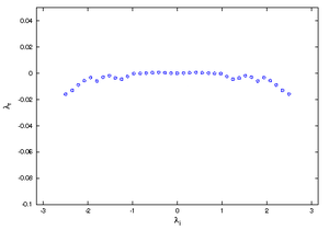
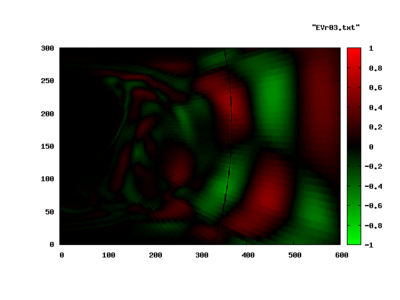
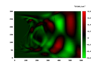
Roughly a third of the spectrum was highly damped (large, negative λr) and is not shown. The dominant shedding mode is shown in the following pictures. The image to the left is the real part, the image to the right, the imaginary part of the Eigenvector.
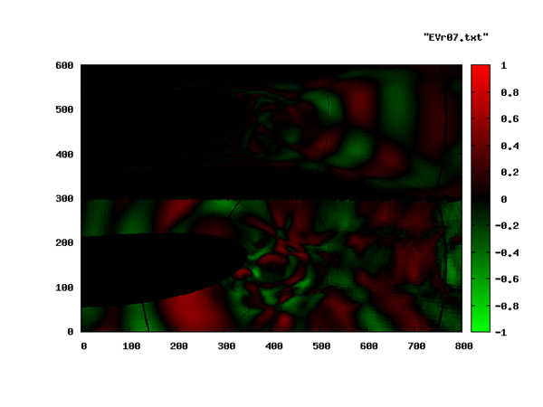
Again, the Entropy-Eigenvector is shown in this pictures. The acoustic contents of the same mode is seen in the bottom half of the next plot. The top half corresponds to the entropy mode as above.
Synthetic Example of a traveling pattern
The DMD analysis assumes a pattern of the form
 where x1 is any of the independent variables of the problem, but has to be selected in advance. Take for example the pattern
With the time as the preselected exponential factor.
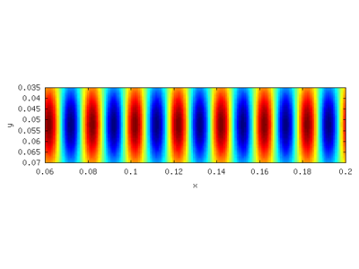
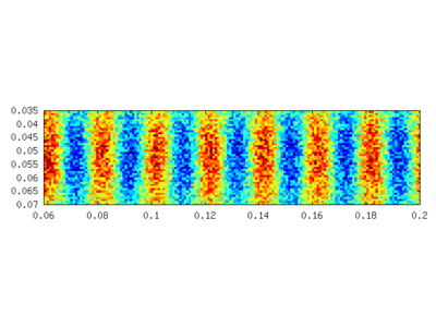
A sample is given in the following figure with ω = 2 * π / 0.1, b = 0.02 and k = 2 * π / b The left picture shows the pattern without, the right with noise added. The amplitude of the random noise is the same as that of the pattern.
A DMD analysis is performed with 21 synthetically generated fields using a time interval Δt = 1 / 90s, limiting the analysis to f = 45Hz.
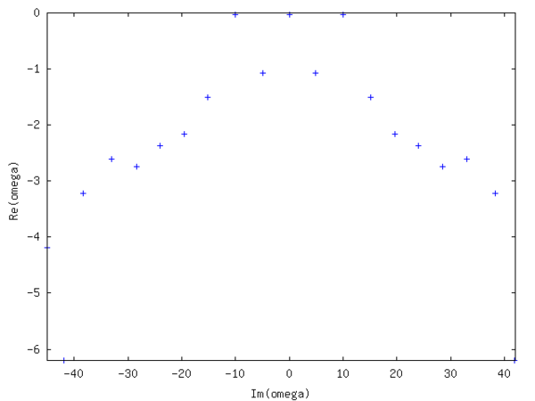
The spectrum is symmetric and shows 3 almost undamped modes (small negative Real part), whereas the other modes are heavily damped. Their numerical values are
 respectively. The real one corresponds to the mean of the field, whereas ω2 / 3 corresponds to the imposed pattern with f = 10Hz. Yielding a relative error of -1/1000. Increasing the noise to 10 times the signal value yields about the same error. The real and imaginary part of one of the latter two Eigenmodes is depicted in the following figure.
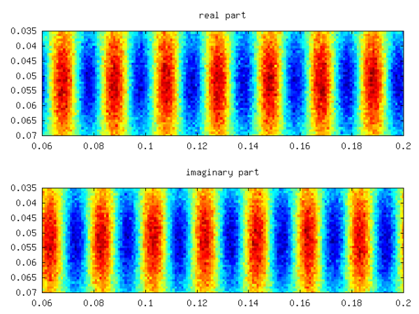
See also
Several other decompositions of experimental data exist. If the governing equations are available, an eigenvalue decomposition might be feasible.
- Eigenvalue decomposition
- Empirical mode decomposition
- POPs and PIPs
- Proper orthogonal decomposition
References
- Hasselmann, K., 1988. POPs and PIPs. The reduction of complex dynamical systems using principal oscillation and interaction patterns. J. Geophys. Res., 93(D9): 10975–10988.
Categories:


Wikimedia Foundation. 2010.