- Delta potential
-
The delta potential is a potential that gives rise to many interesting results in quantum mechanics. It consists of a time-independent Schrödinger equation for a particle in a potential well defined by a Dirac delta function in one dimension.
For those familiar with the particle in a box problem, the delta function potential well is a special case of the finite potential well, and follows as a limit as the depth goes to infinity and the width goes to zero, keeping their product constant.
Contents
Definition

The time-independent Schrödinger equation for the wave function ψ(x) of a particle in one dimension in a potential V(x) is
where ħ is the reduced Planck constant and E is the energy of the particle.
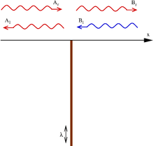
The delta potential is the potential
where δ(x) is the Dirac delta function. It is called a delta potential well if λ is negative and a delta potential barrier if λ is positive. The delta has been defined to occur at the origin for simplicity; a shift in the delta function's argument does not change any of the proceeding results.
Derivation
The potential splits the space in two parts (x < 0 and x > 0). In each of these parts the potential energy is zero, and the Schrödinger equation reduces to
 this is a linear differential equation with constant coefficients whose solutions are linear combinations of eikx and e−ikx, where the wave number k is related to the energy by k = √2mE/ħ. In general, due to the presence of the delta potential in the origin, the coefficients of the solution need not be the same in both half-spaces:
where, in the case of positive energies (real k), eikx represents a wave traveling to the right, and e−ikx one traveling to the left.
Two relations between the coefficients can be found by imposing that the wave function be continuous in the origin (ψ(0) = ψL(0) = ψR(0) = Ar + Al = Br + Bl), and by integrating the Schrödinger equation around x = 0, over an interval [−ε, +ε]:
In the limit as ε → 0, the right-hand side of this equation vanishes; the left-hand side becomes
 [ψ′R(0) − ψ′L(0)] + λψ(0) (Because
 ![\int_{-\epsilon}^{+\epsilon} \psi''(x) \,dx = [\psi'({+\epsilon}) - \psi'({-\epsilon})]](d/64d9dcd5463c1dff229c35c87adc022b.png) ). Substituting the definition of ψ into this expression, we get
). Substituting the definition of ψ into this expression, we getThe boundary conditions thus give the following restrictions on the coefficients
Transmission and reflection (positive energies)
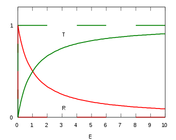 Transmission (T) and reflection (R) probability of a delta potential well. The energy
 is in units of
  . Dashed: classical result. Solid line: quantum mechanics.
For positive energies, the particle is free to move in either half-space: x < 0 or x > 0. It may be scattered at the delta function potential.
The quantum case can be studied in the following situation: a particle incident on the barrier from the left side (Ar). It may be reflected (Al) or transmitted (Br). To find the amplitudes for reflection and transmission for incidence from the left, we put in the above equations Ar = 1 (incoming particle), Al = r (reflection), Bl = 0 (no incoming particle from the right) and Br = t (transmission), and solve for r and t. The result is:
Due to the mirror symmetry of the model, the amplitudes for incidence from the right are the same as those from the left. The result is that there is a non-zero probability
for the particle to be reflected. This does not depend on the sign of λ, that is, a barrier has the same probability of reflecting the particle as a well. This is a significant difference from classical mechanics, where the reflection probability would be 1 for the barrier (the particle simply bounces back), and 0 for the well (the particle passes through the well undisturbed).
Taking this to conclusion, the probability for transmission is:
 .
.
Bound state (negative energy)
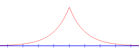
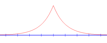 The graph of the bound state wavefunction solution to the delta function potential is continuous everywhere, but its derivative is not at x=0.
In any one-dimensional attractive potential there will be a bound state. To find its energy, note that for E < 0, k = i√2m|E|/ħ = iκ is complex and the wave functions which were oscillating for positive energies in the calculation above, are now exponentially increasing or decreasing functions of x (see above). Requiring that the wave functions do not diverge at infinity eliminates half of the terms: Al = Br = 0. The wave function is then
From the boundary conditions and normalization conditions, it follows that
from which it follows that λ must be negative, that is the bound state only exists for the well, and not for the barrier. The energy of the bound state is then
Remarks and application
The calculation presented above may at first seem unrealistic and hardly useful. However it has proved to be a suitable model for a variety of real-life systems. One such example regards the interfaces between two conducting materials. In the bulk of the materials, the motion of the electrons is quasi free and can be described by the kinetic term in the above Hamiltonian with an effective mass
 . Often the surfaces of such materials are covered with oxide layers or are not ideal for other reasons. This thin, non-conducting layer may then be modeled by a local delta-function potential as above. Electrons may then tunnel from one material to the other giving rise to a current.
The operation of a scanning tunneling microscope (STM) relies on this tunneling effect. In that case, the barrier is due to the air between the tip of the STM and the underlying object. The strength of the barrier is related to the separation being stronger the further apart the two are. For a more general model of this situation, see Finite potential barrier (QM). The delta function potential barrier is the limiting case of the model considered there for very high and narrow barriers.
The above model is one-dimensional while the space around us is three-dimensional. So in fact one should solve the Schrödinger equation in three dimensions. On the other hand, many systems only change along one coordinate direction and are translationally invariant along the others. The Schrödinger equation may then be reduced to the case considered here by an Ansatz for the wave function of the type:
 .
.The delta function model is actually a one-dimensional version of the Hydrogen atom according to the dimensional scaling method developed by the group of Dudley R. Herschbach[1] The delta function model becomes particularly useful with the double-well Dirac Delta function model which represents a one-dimensional version of the Hydrogen molecule ion as shown in the following section.
Double-well Dirac delta function model
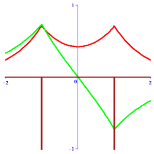 The symmetric and anti-symmetric wavefunctions for the Double-well Dirac delta function model with "internuclear" distance R=2.
The Double-well Dirac delta function model is described by the corresponding Schrödinger equation:
where the potential is now:
where
 is the "internuclear" distance with Dirac delta function (negative) peaks located at
  (shown in brown in the diagram). Keeping in mind the relationship of this model with its three-dimensional molecular counterpart, we use Atomic units and set
  . Here 0 < λ < 1 is a formally adjustable parameter. From the single well case, we can infer the "ansatz" for the solution to be:
Matching of the wavefunction at the Dirac delta function peaks yields the determinant:
Thus, d is found to be governed by the pseudo-quadratic equation:
which has two solutions
 . For the case of equal charges (symmetric homonuclear case), λ = 1 and the pseudo-quadratic reduces to:
The "+" case corresponds to a wave function symmetric about the mid-point (shown in red in the diagram) where A = B and is called gerade. Correspondingly, the "-" case is the wave function that is anti-symmetric about the mid-point where A = − B is called ungerade (shown in green in the diagram). They represent an approximation of the two lowest discrete energy states of the three-dimensional
 and are useful in its analysis. Analytical solutions for the energy eigenvalues for the case of symmetric charges are given by [2]:
where W is the standard Lambert W function. Note that the lowest energy corresponds to the symmetric solution d + . In the case of unequal charges, and for that matter the three-dimensional molecular problem, the solutions are given by a generalization of the Lambert W function (see section on generalization of Lambert W function and references herein).
One of the most interesting cases is when
 which results in d − = 0. Thus, we will have a non-trivial bound state solution that has E = 0. For these specific parameters, there are many interesting properties that occur, one of which is the unusual effect that the Transmission coefficient is unity at zero energy. [3]
See also
- The free particle
- The particle in a box
- The finite potential well
- The particle in a ring
- The particle in a spherically symmetric potential
- The quantum harmonic oscillator
- The hydrogen atom or The hydrogen-like atom
- The ring wave guide
- The particle in a one-dimensional lattice (periodic potential)
- The hydrogen molecular ion
- Holstein–Herring method
Notes
- ^ D.R. Herschbach, J.S. Avery, and O. Goscinski (eds.), Dimensional Scaling in Chemical Physics, Springer, (1992). [1]
- ^ T.C. Scott, J.F. Babb, A. Dalgarno and John D. Morgan III, "The Calculation of Exchange Forces: General Results and Specific Models", J. Chem. Phys., 99, pp. 2841-2854, (1993). [2]
- ^ W. van Dijk and K. A. Kiers, "Time delay in simple one-dimensional systems", Am. J. Phys., 60, pp. 520-527, (1992). [3]
References
- Griffiths, David J. (2005). Introduction to Quantum Mechanics (2nd ed.). Prentice Hall. pp. 68–78. ISBN 0-13-111892-7.
Categories:- Quantum models


![V(x)=-q \left[ \delta (x + \frac{R}{2}) + \lambda \delta (x- \frac{R}{2}) \right]](e/beeea4eb737956089b3f4a2e3932aa74.png)


![d_{\pm} (\lambda )~=~{\textstyle\frac{1}{2}}q (\lambda+1)
\pm {\textstyle\frac{1}{2}}
\left\{ q^2 (1+\lambda )^{2}-4\,\lambda q^2 \lbrack 1-e^{-2d_{\pm }(\lambda
)R}]\right\} ^{1/2}](d/1cdf0b20307ffcb970f913a996bb7a74.png)
![d_{\pm} = q [1 \pm e^{-d_{\pm} R}]](2/1b25bdd9e628549118cff1f2587d7445.png)

Wikimedia Foundation. 2010.