- Coupled map lattice
-
A coupled map lattice (CML) is a dynamical system that models the behavior of non-linear systems (especially partial differential equations). They are predominantly used to qualitatively study the chaotic dynamics of spatially extended systems. This includes the dynamics of spatiotemporal chaos where the number of effective degrees of freedom diverge as the size of the system increases [1]. Features of the CML are discrete time dynamics, discrete underlying spaces (lattices or networks), and real (number or vector), local, continuous state variables [2]. Studied systems include populations, chemical reactions, convection, fluid flow and biological networks. Even recently, CMLs have been applied to computational networks [3] identifying detrimental attack methods and cascading failures.
CML’s are comparable to cellular automata models in terms of their discrete features [4]. However, the value of each site in a cellular automata network is strictly dependent on its neighbor (s) from the previous time step. Each site of the CML is only dependent upon its neighbors relative to the coupling term in the recurrence equation. However, the similarities can be compounded when considering multicomponent dynamical systems.
Contents
Introduction
The modeling of a CML generally incorporates a system of equations (coupled or uncoupled), a finite number of variables, a global or local coupling scheme and the corresponding coupling terms. The dimension of the underlying lattice can exist in infinite dimensions, but for this observation we restrict the lattice to two. Mappings of interest in CMLs generally demonstrate a chaotic behavior. Such maps can be found here: List of chaotic maps.
A logistic mapping demonstrates chaotic behavior, easily identifiable in one dimension for parameter r > 3.57 (see Logistic map). It is graphed across a small lattice and decoupled with respect to neighboring sites. The recurrence equation is homogeneous, albeit randomly seeded. The parameter r is updated every time step (see Figure 1, Enlarge, Summary):
The result is a raw form of chaotic behavior in a map lattice. The range of the function is bounded so similar contours through the lattice is expected. However, there are no significant spatial correlations or pertinent fronts to the chaotic behavior. No obvious order is apparent.
For a basic coupling, we consider a 'single neighbor' coupling where the value at any given site s is mapped recursively with respect to itself and the neighboring site s − 1. The coupling parameter
 is equally weighted.
Even though each native recursion is chaotic, a more solid form develops in the evolution. Elongated convective spaces persist throughout the lattice (see Figure 2).


Figure 1: An uncoupled logistic map lattice
with random seeding over forty iterates.Figure 2: A CML with a single-neighbor
coupling scheme taken over forty iterates.History
CMLs were first introduced in the mid 1980’s through a series of closely released publications [5][6][7][8]. Kapral used CMLs for modeling chemical spatial phenomena. Kuznetsov sought to apply CMLs to electrical circuitry by developing a renormalization group approach (similar to Feigenbaum's universality to spatially extended systems). Kaneko's focus was more broad and he is still known as the most active researcher in this area [9].The most examined CML model was introduced by Kaneko in 1983 where the recurrence equation is as follows:
where
 and f is a real mapping.
The applied CML strategy was as follows:
- Choose a set of field variables on the lattice at a macroscopic level. The dimension (not limited by the CML system) should be chosen to correspond to the physical space being researched.
- Decompose the process (underlying the phenomena) into independent components.
- Replace each component by a nonlinear transformation of field variables on each lattice point and the coupling term on suitable, chosen neighbors.
- Carry out each unit dynamics ("procedure") successively.
Classification
The CML system evolves through discrete time by a mapping on vector sequences. These mappings are a recursive function of two competing terms: an individual nonlinear reaction, and a spatial interaction (coupling) of variable intensity. CMLs can be classified by the strength of this coupling parameter(s).
Much of the current published work in CMLs is based in weak coupled systems [10] where diffeomorphism of the state space close to identity are studied. Weak coupling with monotonic (bistable) dynamical regimes demonstrate spatial chaos phenomena and are popular in neural models [11]. Weak coupling unimodal maps are characterized by their stable periodic points and are used by genetic regulatory network models. Space-time chaotic phenomena can be demonstrated from chaotic mappings subject to weak coupling coefficients and are popular in phase transition phenomena models.
Intermediate and strong coupling interactions are less prolific areas of study. Intermediate interactions are studied with respect to fronts and traveling waves, riddled basins, riddled bifurcations, clusters and non-unique phases. Strong coupling interactions are most well known to model synchronization effects of dynamic spatial systems such as the Kuramoto model.
These classifications do not reflect the local or global (GMLs [12] )coupling nature of the interaction. Nor do they consider the frequency of the coupling which can exist as a degree of freedom in the system [13]. Finally, they do not distinguish between sizes of the underlying space or boundary conditions.
Surprisingly the dynamics of CMLs have little to do with the local maps that constitute their elementary components. With each model a rigorous mathematical investigation is needed to identify a chaotic state (beyond visual interpretation). Rigorous proofs have been performed to this effect. By example: the existence of space-time chaos in weak space interactions of one-dimensional maps with strong statistical properties was proven by Bunimovich and Sinai in 1988 [14]. Similar proofs exist for weakly hyperbolic maps under the same conditions.
Unique CML qualitative classes
CMLs have revealed novel qualitative universality classes in (CML) phenomenology. Such classes include:
- Spatial bifurcation and frozen chaos
- Pattern Selection
- Selection of zig-zag patterns and chaotic diffusion of defects
- Spatio-temporal intermittency
- Soliton turbulence
- Global traveling waves generated by local phase slips
- Spatial bifurcation to down-flow in open flow systems.
Visual phenomena
The unique qualitative classes listed above can be visualized. By applying the Kaneko 1983 model to the logistic f(xn) = 1 − ax2 map, several of the CML qualitative classes may be observed. These are demonstrated below, note the unique parameters:
Frozen Chaos Pattern Selection Chaotic Brownian Motion of Defect 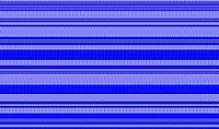
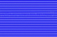
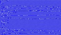
Figure 1: Sites are divided into non-uniform clusters, where the divided patterns are regarded as attractors. Sensitivity to initial conditions exist relative to a < 1.5. Figure 2: Near uniform sized clusters (a = 1.71, ε = 0.4). Figure 3: Deflects exist in the system and fluctuate chaotically akin to Brownian motion (a = 1.85, ε = 0.1). Defect Turbulence Spatiotemporal Intermittency I Spatiotemporal Intermittency II 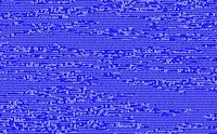
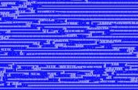
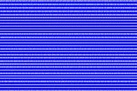
Figure 4: Many defects are generated and turbulently collide (a = 1.895, ε = 0.1). Figure 5: Each site transits between a coherent state and chaotic state intermittently (a = 1.75, ε = 0.6), Phase I. Figure 6: The coherent state, Phase II. Fully Developed Spatiotemporal Chaos Traveling Wave 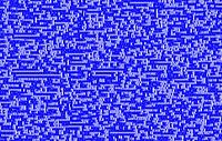
Figure 7: Most sites independently oscillate chaotically (a = 2.00, ε = 0.3). Figure 8: The wave of clusters travels at 'low' speeds (a = 1.47, ε = 0.5). Quantitative analysis quantifiers
Coupled map lattices being a prototype of spatially extended systems easy to simulate have represented a benchmark for the definition and introduction of many indicators of spatio-temporal chaos, the most relevant ones are
- The power spectrum in space and time
- Lyapunov spectra[15]
- Dimension density
- Kolmogorov–Sinai entropy density
- Distributions of patterns
- Pattern entropy
- Propagation speed of finite and infinitesimal disturbance
- Mutual information and correlation in space-time
- Lyapunov exponents, localization of Lyapunov vectors
- Comoving and sub-space time Lyapunov exponents.
- Spatial and temporal Lyapunov exponents [16]
See also
- Dynamical systems
- Chaos theory
- Lyapunov exponent
- Cellular automata
References
- ^ Kaneko, Kunihiko. "Overview of Coupled Map Lattices." Chaos 2, Num3(1992): 279.
- ^ Chazottes, Jean-René, and Bastien Fernandez. Dynamics of Coupled Map Lattices and of Related Spatially Extended Systems. Springer, 2004. pgs 1–4
- ^ Xu, Jian. Wang, Xioa Fan. " Cascading failures in scale-free coupled map lattices." IEEE International Symposium on Circuits and Systems “ ISCAS Volume 4, (2005): 3395–3398.
- ^ R. Badii and A. Politi, Complexity: Hierarchical Structures and Scaling in Physics (Cambridge University Press,Cambridge, England, 1997).
- ^ K. Kaneko, Prog. Theor. Phys. 72, 480 (1984)
- ^ I. waller and R. Kapral; Phys. Rev. A 30 2047 (1984)
- ^ J. Crutchfield, Phyisca D 10, 229 (1984)
- ^ S. P.Kuznetsov and A. S. Pikovsky, Izvestija VUS, Radiofizika 28, 308 (1985)
- ^ http://chaos.c.u-tokyo.ac.jp/
- ^ Lectures from the school-forum (CML 2004) held in Paris, June 21{July 2, 2004. Edited by J.-R. Chazottes and B. Fernandez. Lecture Notes in Physics, 671. Springer, Berlin (2005)
- ^ Nozawa, Hiroshi. "A neural network model." Chaos 2, Num3(1992): 377.
- ^ Ho, Ming-Ching. Hung, Yao-Chen. Jiang, I-Min. "Phase synchronization in inhomogenous globally coupled map lattices. Physics Letter A. 324 (2004) 450–457. [1]
- ^ http://www.mat.uniroma2.it/~liverani/Lavori/live0803.pdf
- ^ L.A. Bunimovich and Ya. G. Sinai. "Nonlinearity" Vol. 1 pg 491 (1988)
- ^ Lyapunov Spectra of Coupled Map Lattices, S. Isola, A. Politi, S. Ruffo, and A. Torcini
- ^ S. Lepri, A. Politi and A. Torcini Chronotopic Lyapunov Analysis: (I) a Detailed Characterization of 1D Systems, J. Stat. Phys., 82 5/6 (1996) 1429.
Further reading
- Google Library (2005). Dynamics of Coupled Map Lattices. Springer. ISBN 9783540242895. Archived from the original on 2008-03-29. http://books.google.com/books?id=a63Q8DhKA44C&dq=coupled+map+lattices&source=gbs_summary_s&hl=en.
- Shawn D. Pethel, Ned J. Corron, and Erik Bollt. "Symbolic Dynamics of Coupled Map Lattices". Physical Review Letters. Archived from the original on 2008-03-29. http://people.clarkson.edu/~bolltem/Papers/PhysRevLett_96_034105PethelCorronBollt.pdf.
- E. Atlee Jackson, Perspectives of Nonlinear Dynamics: Volume 2, Cambridge University Press, 1991, ISBN 0521426332, http://books.google.com/books?id=M2E0AAAAIAAJ&source=gbs_ViewAPI
- H.G, Schuster and W. Just, Deterministic Chaos, John Wiley and Sons Ltd, 2005, ISBN 3527404155, http://www.whsmith.co.uk/CatalogAndSearch/ProductDetails.aspx?productID=9783527404155
- Introduction to Chaos and Nonlinear Dynamics
External links
- Kaneko Laboratory
- Institut Henri Poincaré, Paris, June 21 – July 2, 2004
- Istituto dei Sistemi Complessi, Florence, Italy
Software
Categories:- Physics
- Chaos theory
- Nonlinear dynamics

![\qquad x_{n+1} = (\epsilon)[r x_n (1-x_n)]_s + (1-\epsilon)[r x_n (1-x_n)]_{s-1}](8/54896ec4f9c277a99ae66bd07fdf29d1.png)


![u_s^{t+1} = (1-\varepsilon)f(u_s^t)+\frac{\varepsilon}{2}\left(f(u_{s+1}^t)+f(u_{s-1}^t) \right) \ \ \ t\in \mathbb{N},\ \varepsilon \in [0,1]](3/bf36182252573bd09b1bcfd1f5af662a.png)


Wikimedia Foundation. 2010.