Cooley–Tukey FFT algorithm

The Cooley–Tukey algorithm, named after J.W. Cooley and John Tukey, is the most common fast Fourier transform (FFT) algorithm. It re-expresses the discrete Fourier transform (DFT) of an arbitrary composite size N = N₁N₂ in terms of smaller DFTs of sizes N₁ and N₂, recursively, in order to reduce the computation time to O(N log N) for highly-composite N (smooth numbers). Because of the algorithm's importance, specific variants and implementation styles have become known by their own names, as described below.

Because the Cooley-Tukey algorithm breaks the DFT into smaller DFTs, it can be combined arbitrarily with any other algorithm for the DFT. For example, Rader's or Bluestein's algorithm can be used to handle large prime factors that cannot be decomposed by Cooley–Tukey, or the prime-factor algorithm can be exploited for greater efficiency in separating out relatively prime factors.

See also the fast Fourier transform for information on other FFT algorithms, specializations for real and/or symmetric data, and accuracy in the face of finite floating-point precision.

History

This algorithm, including its recursive application, was invented around 1805 by Carl Friedrich Gauss, who used it to interpolate the trajectories of the asteroids Pallas and Juno, but his work was not widely recognized (being published only posthumously and in neo-Latin).^[1][2] Gauss did not analyze the asymptotic computational time, however. Various limited forms were also rediscovered several times throughout the 19th and early 20th centuries.^[2] FFTs became popular after J. W. Cooley of IBM and John W. Tukey of Princeton published a paper in 1965 reinventing the algorithm and describing how to perform it conveniently on a computer.^[3]

Tukey reportedly came up with the idea during a meeting of a US presidential advisory committee discussing ways to detect nuclear-weapon tests in the Soviet Union.^[4][5] Another participant at that meeting, Richard Garwin of IBM, recognized the potential of the method and put Tukey in touch with Cooley, who implemented it for a different (and less-classified) problem: analyzing 3d crystallographic data (see also: multidimensional FFTs). Cooley and Tukey subsequently published their joint paper, and wide adoption quickly followed.

The fact that Gauss had described the same algorithm (albeit without analyzing its asymptotic cost) was not realized until several years after Cooley and Tukey's 1965 paper.^[2] Their paper cited as inspiration only work by I. J. Good on what is now called the prime-factor FFT algorithm (PFA);^[3] although Good's algorithm was initially mistakenly thought to be equivalent to the Cooley–Tukey algorithm, it was quickly realized that PFA is a quite different algorithm (only working for sizes that have relatively prime factors and relying on the Chinese Remainder Theorem, unlike the support for any composite size in Cooley–Tukey).^[6]

The radix-2 DIT case

A radix-2 decimation-in-time (DIT) FFT is the simplest and most common form of the Cooley–Tukey algorithm, although highly optimized Cooley–Tukey implementations typically use other forms of the algorithm as described below. Radix-2 DIT divides a DFT of size N into two interleaved DFTs (hence the name "radix-2") of size N/2 with each recursive stage.

The discrete Fourier transform (DFT) is defined by the formula:

$X_k = \sum_{n=0}^{N-1} x_n e^{-\frac{2\pi i}{N} nk},$

where k is an integer ranging from 0 to N − 1.

Radix-2 DIT first computes the DFTs of the even-indexed inputs $x_{2m} \$ ($x_0, x_2, \ldots, x_{N-2}$) and of the odd-indexed inputs $x_{2m+1} \$ ($x_1, x_3, \ldots, x_{N-1}$), and then combines those two results to produce the DFT of the whole sequence. This idea can then be performed recursively to reduce the overall runtime to O(N log N). This simplified form assumes that N is a power of two; since the number of sample points N can usually be chosen freely by the application, this is often not an important restriction.

The Radix-2 DIT algorithm rearranges the DFT of the function x_n into two parts: a sum over the even-numbered indices n = 2m and a sum over the odd-numbered indices n = 2m + 1:

$\begin{matrix} X_k & = & \sum \limits_{m=0}^{N/2-1} x_{2m} e^{-\frac{2\pi i}{N} (2m)k} + \sum \limits_{m=0}^{N/2-1} x_{2m+1} e^{-\frac{2\pi i}{N} (2m+1)k}. \end{matrix}$

One can factor a common multiplier $e^{-\frac{2\pi i}{N}k}$ out of the second sum, as shown in the equation below. It is then clear that the two sums are the DFT of the even-indexed part x_2m and the DFT of odd-indexed part x_{2m + 1} of the function x_n. Denote the DFT of the Even-indexed inputs x_2m by E_k and the DFT of the Odd-indexed inputs x_{2m + 1} by O_k and we obtain:

$\begin{matrix} X_k= \underbrace{\sum \limits_{m=0}^{N/2-1} x_{2m} e^{-\frac{2\pi i}{N/2} mk}}_{\mathrm{DFT\;of\;even-indexed\;part\;of\;} x_m} {} + e^{-\frac{2\pi i}{N}k} \underbrace{\sum \limits_{m=0}^{N/2-1} x_{2m+1} e^{-\frac{2\pi i}{N/2} mk}}_{\mathrm{DFT\;of\;odd-indexed\;part\;of\;} x_m} = E_k + e^{-\frac{2\pi i}{N}k} O_k. \end{matrix}$

However, these smaller DFTs have a length of N/2, so we need compute only N/2 outputs: thanks to the periodicity properties of the DFT, the outputs for $N/2 \leq k < N$ from a DFT of length N/2 are identical to the outputs for $0\leq k < N/2$. That is, E_{k + N / 2} = E_k and O_{k + N / 2} = O_k. The phase factor exp[ − 2πik / N] (called a twiddle factor) obeys the relation: exp[ − 2πi(k + N / 2) / N] = e ^{− πi}exp[ − 2πik / N] = − exp[ − 2πik / N], flipping the sign of the O_{k + N / 2} terms. Thus, the whole DFT can be calculated as follows:

$\begin{matrix} X_k & = & \left\{ \begin{matrix} E_k + e^{-\frac{2\pi i}{N}k} O_k & \mbox{if } k < N/2 \\ \\ E_{k-N/2} - e^{-\frac{2\pi i}{N} (k-N/2)} O_{k-N/2} & \mbox{if } k \geq N/2. \end{matrix} \right. \end{matrix}$

This result, expressing the DFT of length N recursively in terms of two DFTs of size N/2, is the core of the radix-2 DIT fast Fourier transform. The algorithm gains its speed by re-using the results of intermediate computations to compute multiple DFT outputs. Note that final outputs are obtained by a +/− combination of E_k and O_kexp( − 2πik / N), which is simply a size-2 DFT (sometimes called a butterfly in this context); when this is generalized to larger radices below, the size-2 DFT is replaced by a larger DFT (which itself can be evaluated with an FFT).

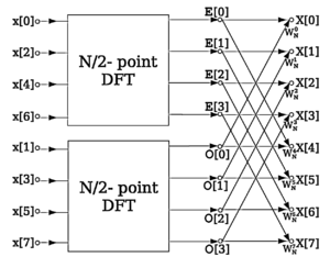Data flow diagram for N=8: a decimation-in-time radix-2 FFT breaks a length-N DFT into two length-N/2 DFTs followed by a combining stage consisting of many size-2 DFTs called "butterfly" operations (so-called because of the shape of the data-flow diagrams).

This process is an example of the general technique of divide and conquer algorithms; in many traditional implementations, however, the explicit recursion is avoided, and instead one traverses the computational tree in breadth-first fashion.

The above re-expression of a size-N DFT as two size-N/2 DFTs is sometimes called the Danielson–Lanczos lemma, since the identity was noted by those two authors in 1942^[7] (influenced by Runge's 1903 work^[2]). They applied their lemma in a "backwards" recursive fashion, repeatedly doubling the DFT size until the transform spectrum converged (although they apparently didn't realize the linearithmic asymptotic complexity they had achieved). The Danielson–Lanczos work predated widespread availability of computers and required hand calculation (possibly with mechanical aids such as adding machines); they reported a computation time of 140 minutes for a size-64 DFT operating on real inputs to 3–5 significant digits. Cooley and Tukey's 1965 paper reported a running time of 0.02 minutes for a size-2048 complex DFT on an IBM 7094 (probably in 36-bit single precision, ~8 digits).^[3] Rescaling the time by the number of operations, this corresponds roughly to a speedup factor of around 800,000. (To put the time for the hand calculation in perspective, 140 minutes for size 64 corresponds to an average of at most 16 seconds per floating-point operation, around 20% of which are multiplications.)

Pseudocode

In pseudocode, the above process could be written:^[8]

X0,...,N−1 ← ditfft2(x, N, s):             DFT of (x0, xs, x2s, ..., x(N-1)s):
    if N = 1 then
        X0 ← x0                                      trivial size-1 DFT base case
    else
        X0,...,N/2−1 ← ditfft2(x, N/2, 2s)             DFT of (x0, x2s, x4s, ...)
        XN/2,...,N−1 ← ditfft2(x+s, N/2, 2s)           DFT of (xs, xs+2s, xs+4s, ...)
        for k = 0 to N/2−1                           combine DFTs of two halves into full DFT:
            t ← Xk
            Xk ← t + exp(−2πi k/N) Xk+N/2
            Xk+N/2 ← t − exp(−2πi k/N) Xk+N/2
        endfor
    endif

Here, ditfft2(x,N,1), computes X=DFT(x) out-of-place by a radix-2 DIT FFT, where N is an integer power of 2 and s=1 is the stride of the input x array. x+s denotes the array starting with x_s.

(The results are in the correct order in X and no further bit-reversal permutation is required; the often-mentioned necessity of a separate bit-reversal stage only arises for certain in-place algorithms, as described below.)

High-performance FFT implementations make many modifications to the implementation of such an algorithm compared to this simple pseudocode. For example, one can use a larger base case than N=1 to amortize the overhead of recursion, the twiddle factors exp(−2πi k/N) can be precomputed, and larger radices are often used for cache reasons; these and other optimizations together can improve the performance by an order of magnitude or more.^[8] (In many textbook implementations the depth-first recursion is eliminated entirely in favor of a nonrecursive breadth-first approach, although depth-first recursion has been argued to have better memory locality.^[8][9]) Several of these ideas are described in further detail below.

General factorizations

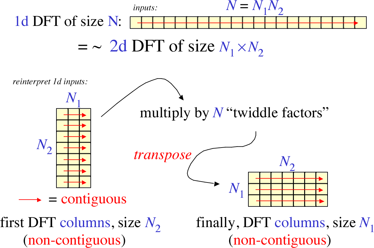
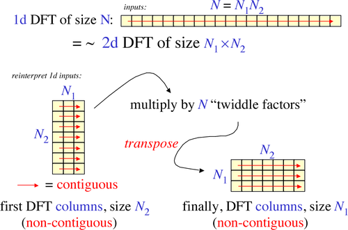The basic step of the Cooley–Tukey FFT for general factorizations can be viewed as re-interpreting a 1d DFT as something like a 2d DFT. The 1d input array of length N = N₁N₂ is reinterpreted as a 2d N₁×N₂ matrix stored in column-major order. One performs smaller 1d DFTs along the N₂ direction (the non-contiguous direction), then multiplies by phase factors (twiddle factors), and finally performs 1d DFTs along the N₁ direction, at some point transposing the matrix. This is done recursively for the smaller transforms.

More generally, Cooley–Tukey algorithms recursively re-express a DFT of a composite size N = N₁N₂ as:^[10]

1. Perform N₁ DFTs of size N₂.
2. Multiply by complex roots of unity called twiddle factors.
3. Perform N₂ DFTs of size N₁.

Typically, either N₁ or N₂ is a small factor (not necessarily prime), called the radix (which can differ between stages of the recursion). If N₁ is the radix, it is called a decimation in time (DIT) algorithm, whereas if N₂ is the radix, it is decimation in frequency (DIF, also called the Sande-Tukey algorithm). The version presented above was a radix-2 DIT algorithm; in the final expression, the phase multiplying the odd transform is the twiddle factor, and the +/- combination (butterfly) of the even and odd transforms is a size-2 DFT. (The radix's small DFT is sometimes known as a butterfly, so-called because of the shape of the dataflow diagram for the radix-2 case.)

There are many other variations on the Cooley–Tukey algorithm. Mixed-radix implementations handle composite sizes with a variety of (typically small) factors in addition to two, usually (but not always) employing the O(N²) algorithm for the prime base cases of the recursion [it is also possible to employ an N log N algorithm for the prime base cases, such as Rader's or Bluestein's algorithm]. Split radix merges radices 2 and 4, exploiting the fact that the first transform of radix 2 requires no twiddle factor, in order to achieve what was long the lowest known arithmetic operation count for power-of-two sizes,^[10] although recent variations achieve an even lower count.^[11][12] (On present-day computers, performance is determined more by cache and CPU pipeline considerations than by strict operation counts; well-optimized FFT implementations often employ larger radices and/or hard-coded base-case transforms of significant size.^[13]) Another way of looking at the Cooley–Tukey algorithm is that it re-expresses a size N one-dimensional DFT as an N₁ by N₂ two-dimensional DFT (plus twiddles), where the output matrix is transposed. The net result of all of these transpositions, for a radix-2 algorithm, corresponds to a bit reversal of the input (DIF) or output (DIT) indices. If, instead of using a small radix, one employs a radix of roughly √N and explicit input/output matrix transpositions, it is called a four-step algorithm (or six-step, depending on the number of transpositions), initially proposed to improve memory locality,^[14][15] e.g. for cache optimization or out-of-core operation, and was later shown to be an optimal cache-oblivious algorithm.^[16]

The general Cooley–Tukey factorization rewrites the indices k and n as k = N₂k₁ + k₂ and n = N₁n₂ + n₁, respectively, where the indices k_a and n_a run from 0..N_a-1 (for a of 1 or 2). That is, it re-indexes the input (n) and output (k) as N₁ by N₂ two-dimensional arrays in column-major and row-major order, respectively; the difference between these indexings is a transposition, as mentioned above. When this re-indexing is substituted into the DFT formula for nk, the N₁n₂N₂k₁ cross term vanishes (its exponential is unity), and the remaining terms give

$X_{N_2 k_1 + k_2} = \sum_{n_1=0}^{N_1-1} \sum_{n_2=0}^{N_2-1} x_{N_1 n_2 + n_1} e^{-\frac{2\pi i}{N_1 N_2} \cdot (N_1 n_2 + n_1) \cdot (N_2 k_1 + k_2) }$

$= \sum_{n_1=0}^{N_1-1} \left[ e^{-\frac{2\pi i}{N} n_1 k_2 } \right] \left( \sum_{n_2=0}^{N_2-1} x_{N_1 n_2 + n_1} e^{-\frac{2\pi i}{N_2} n_2 k_2 } \right) e^{-\frac{2\pi i}{N_1} n_1 k_1 }$

where each inner sum is a DFT of size N₂, each outer sum is a DFT of size N₁, and the [...] bracketed term is the twiddle factor.

An arbitrary radix r (as well as mixed radices) can be employed, as was shown by both Cooley and Tukey^[3] as well as Gauss (who gave examples of radix-3 and radix-6 steps).^[2] Cooley and Tukey originally assumed that the radix butterfly required O(r²) work and hence reckoned the complexity for a radix r to be O(r² N/r log_rN) = O(N log₂(N) r/log₂r); from calculation of values of r/log₂r for integer values of r from 2 to 12 the optimal radix is found to be 3 (the closest integer to e, which minimizes r/log₂r).^[3][17] This analysis was erroneous, however: the radix-butterfly is also a DFT and can be performed via an FFT algorithm in O(r log r) operations, hence the radix r actually cancels in the complexity O(r log(r) N/r log_rN), and the optimal r is determined by more complicated considerations. In practice, quite large r (32 or 64) are important in order to effectively exploit e.g. the large number of processor registers on modern processors,^[13] and even an unbounded radix r=√N also achieves O(N log N) complexity and has theoretical and practical advantages for large N as mentioned above.^[14][15][16]

Data reordering, bit reversal, and in-place algorithms

Although the abstract Cooley–Tukey factorization of the DFT, above, applies in some form to all implementations of the algorithm, much greater diversity exists in the techniques for ordering and accessing the data at each stage of the FFT. Of special interest is the problem of devising an in-place algorithm that overwrites its input with its output data using only O(1) auxiliary storage.

The most well-known reordering technique involves explicit bit reversal for in-place radix-2 algorithms. Bit reversal is the permutation where the data at an index n, written in binary with digits b₄b₃b₂b₁b₀ (e.g. 5 digits for N=32 inputs), is transferred to the index with reversed digits b₀b₁b₂b₃b₄ . Consider the last stage of a radix-2 DIT algorithm like the one presented above, where the output is written in-place over the input: when E_k and O_k are combined with a size-2 DFT, those two values are overwritten by the outputs. However, the two output values should go in the first and second halves of the output array, corresponding to the most significant bit b₄ (for N=32); whereas the two inputs E_k and O_k are interleaved in the even and odd elements, corresponding to the least significant bit b₀. Thus, in order to get the output in the correct place, these two bits must be swapped in the input. If you include all of the recursive stages of a radix-2 DIT algorithm, all the bits must be swapped and thus one must pre-process the input with a bit reversal to get in-order output. Correspondingly, the reversed (dual) algorithm is radix-2 DIF, and this takes in-order input and produces bit-reversed output, requiring a bit-reversal post-processing step. Alternatively, some applications (such as convolution) work equally well on bit-reversed data, so one can do radix-2 DIF without bit reversal, followed by processing, followed by the radix-2 DIT inverse DFT without bit reversal to produce final results in the natural order.

Many FFT users, however, prefer natural-order outputs, and a separate, explicit bit-reversal stage can have a non-negligible impact on the computation time,^[13] even though bit reversal can be done in O(N) time and has been the subject of much research.^[18][19][20] Also, while the permutation is a bit reversal in the radix-2 case, it is more generally an arbitrary (mixed-base) digit reversal for the mixed-radix case, and the permutation algorithms become more complicated to implement. Moreover, it is desirable on many hardware architectures to re-order intermediate stages of the FFT algorithm so that they operate on consecutive (or at least more localized) data elements. To these ends, a number of alternative implementation schemes have been devised for the Cooley–Tukey algorithm that do not require separate bit reversal and/or involve additional permutations at intermediate stages.

The problem is greatly simplified if it is out-of-place: the output array is distinct from the input array or, equivalently, an equal-size auxiliary array is available. The Stockham auto-sort algorithm^[21] performs every stage of the FFT out-of-place, typically writing back and forth between two arrays, transposing one "digit" of the indices with each stage, and has been especially popular on SIMD architectures.^[22] Even greater potential SIMD advantages (more consecutive accesses) have been proposed for the Pease algorithm,^[23] which also reorders out-of-place with each stage, but this method requires separate bit/digit reversal and O(N log N) storage. One can also directly apply the Cooley–Tukey factorization definition with explicit (depth-first) recursion and small radices, which produces natural-order out-of-place output with no separate permutation step (as in the pseudocode above) and can be argued to have cache-oblivious locality benefits on systems with hierarchical memory.^[9][13][24]

A typical strategy for in-place algorithms without auxiliary storage and without separate digit-reversal passes involves small matrix transpositions (which swap individual pairs of digits) at intermediate stages, which can be combined with the radix butterflies to reduce the number of passes over the data.^{[13][25][26][27][28]}

References

1. ^ Gauss, Carl Friedrich, "Nachlass: Theoria interpolationis methodo nova tractata", Werke, Band 3, 265–327 (Königliche Gesellschaft der Wissenschaften, Göttingen, 1866)
2. ^ ^{a b c d e} Heideman, M. T., D. H. Johnson, and C. S. Burrus, "Gauss and the history of the fast Fourier transform," IEEE ASSP Magazine, 1, (4), 14–21 (1984)
3. ^ ^{a b c d e} Cooley, James W., and John W. Tukey, "An algorithm for the machine calculation of complex Fourier series," Math. Comput. 19, 297–301 (1965). doi:10.2307/2003354
4. ^ Cooley, James W., Peter A. W. Lewis, and Peter D. Welch, "Historical notes on the fast Fourier transform," IEEE Trans. on Audio and Electroacoustics 15 (2), 76–79 (1967).
5. ^ Rockmore, Daniel N. , Comput. Sci. Eng. 2 (1), 60 (2000). The FFT — an algorithm the whole family can use Special issue on "top ten algorithms of the century "[1]
6. ^ James W. Cooley, Peter A. W. Lewis, and Peter W. Welch, "Historical notes on the fast Fourier transform," Proc. IEEE, vol. 55 (no. 10), p. 1675–1677 (1967).
7. ^ Danielson, G. C., and C. Lanczos, "Some improvements in practical Fourier analysis and their application to X-ray scattering from liquids," J. Franklin Inst. 233, 365–380 and 435–452 (1942).
8. ^ ^{a b c} S. G. Johnson and M. Frigo, “Implementing FFTs in practice,” in Fast Fourier Transforms (C. S. Burrus, ed.), ch. 11, Rice University, Houston TX: Connexions, September 2008.
9. ^ ^{a b} Singleton, Richard C. (1967). "On computing the fast Fourier transform". Commun. of the ACM 10 (10): 647–654. doi:10.1145/363717.363771. 
10. ^ ^{a b} Duhamel, P., and M. Vetterli, "Fast Fourier transforms: a tutorial review and a state of the art," Signal Processing 19, 259–299 (1990)
11. ^ Lundy, T., and J. Van Buskirk, "A new matrix approach to real FFTs and convolutions of length 2^k," Computing 80, 23-45 (2007).
12. ^ Johnson, S. G., and M. Frigo, "A modified split-radix FFT with fewer arithmetic operations," IEEE Trans. Signal Processing 55 (1), 111–119 (2007).
13. ^ ^{a b c d e} Frigo, M.; Johnson, S. G. (2005). "The Design and Implementation of FFTW3". Proceedings of the IEEE 93 (2): 216–231. doi:10.1109/JPROC.2004.840301. http://fftw.org/fftw-paper-ieee.pdf. 
14. ^ ^{a b} Gentleman W. M., and G. Sande, "Fast Fourier transforms—for fun and profit," Proc. AFIPS 29, 563–578 (1966).
15. ^ ^{a b} Bailey, David H., "FFTs in external or hierarchical memory," J. Supercomputing 4 (1), 23–35 (1990)
16. ^ ^{a b} M. Frigo, C.E. Leiserson, H. Prokop, and S. Ramachandran. Cache-oblivious algorithms. In Proceedings of the 40th IEEE Symposium on Foundations of Computer Science (FOCS 99), p.285-297. 1999. Extended abstract at IEEE, at Citeseer.
17. ^ Cooley, J. W., P. Lewis and P. Welch, "The Fast Fourier Transform and its Applications", IEEE Trans on Education 12, 1, 28-34 (1969)
18. ^ Karp, Alan H. (1996). "Bit reversal on uniprocessors". SIAM Review 38 (1): 1–26. doi:10.1137/1038001. JSTOR 2132972. 
19. ^ Carter, Larry; Gatlin, Kang Su (1998). "Towards an optimal bit-reversal permutation program". Proc. 39th Ann. Symp. on Found. of Comp. Sci. (FOCS): 544–553. doi:10.1109/SFCS.1998.743505. 
20. ^ Rubio, M.; Gómez, P.; Drouiche, K. (2002). "A new superfast bit reversal algorithm". Intl. J. Adaptive Control and Signal Processing 16 (10): 703–707. doi:10.1002/acs.718. 
21. ^ Stockham, T. G. (1966). "High speed convolution and correlation". Spring Joint Computer Conference, Proc. AFIPS 28: 229–233. 
22. ^ Swarztrauber, P. N. (1982). "Vectorizing the FFTs". In Rodrigue, G.. Parallel Computations. New York: Academic Press. pp. 51–83. ISBN 0125921012. 
23. ^ Pease, M. C. (1968). "An adaptation of the fast Fourier transform for parallel processing". J. ACM 15 (2): 252–264. doi:10.1145/321450.321457. 
24. ^ Frigo, Matteo; Johnson, Steven G.. "FFTW". http://www.fftw.org/.  A free (GPL) C library for computing discrete Fourier transforms in one or more dimensions, of arbitrary size, using the Cooley–Tukey algorithm
25. ^ Johnson, H. W.; Burrus, C. S. (1984). "An in-place in-order radix-2 FFT". Proc. ICASSP: 28A.2.1–28A.2.4. 
26. ^ Temperton, C. (1991). "Self-sorting in-place fast Fourier transform". SIAM J. Sci. Stat. Comput. 12 (4): 808–823. doi:10.1137/0912043. 
27. ^ Qian, Z.; Lu, C.; An, M.; Tolimieri, R. (1994). "Self-sorting in-place FFT algorithm with minimum working space". IEEE Trans. ASSP 52 (10): 2835–2836. doi:10.1109/78.324749. 
28. ^ Hegland, M. (1994). "A self-sorting in-place fast Fourier transform algorithm suitable for vector and parallel processing". Numerische Mathematik 68 (4): 507–547. doi:10.1007/s002110050074. 

External links

• a simple, pedagogical radix-2 Cooley–Tukey FFT algorithm in C++.
• KISSFFT: a simple mixed-radix Cooley–Tukey implementation in C (open source)