- Continuous-repayment mortgage
-
Analogous to continuous compounding, a continuous annuity[1][2] is an ordinary annuity in which the payment interval is narrowed indefinitely. A (theoretical) continuous repayment mortgage is a mortgage loan paid by means of a continuous annuity.
Mortgages (i.e., mortgage loans) are generally settled over a period of years by a series of fixed regular payments commonly referred to as an annuity. Each payment accumulates compound interest from time of deposit to the end of the mortgage timespan at which point the sum of the payments with their accumulated interest equals the value of the loan with interest compounded over the entire timespan. Given loan P0, per period interest rate i, number of periods n and fixed per period payment x, the end of term balancing equation is:
 Gold pour – an illustration of literal cash "flow".
In a (theoretical) continuous-repayment mortgage the payment interval is narrowed indefinitely until the discrete interval process becomes continuous and the fixed interval payments become – in effect – a literal cash "flow" at a fixed annual rate. In this case, given loan P0, annual interest rate r, loan timespan T (years) and annual rate Ma, the infinitesimal cash flow elements Maδt accumulate continuously compounded interest from time t to the end of the loan timespan at which point the balancing equation is:
Summation of the cash flow elements and accumulated interest is effected by integration as shown. It is assumed that compounding interval and payment interval are equal – i.e., compounding of interest always occurs at the same time as payment is deducted.[5]
Within the timespan of the loan the time continuous mortgage balance function obeys a first order linear differential equation (LDE)[6] and an alternative derivation thereof may be obtained by solving the LDE using the method of Laplace transforms.
Application of the equation yields a number of results relevant to the financial process which it describes. Although this article focuses primarily on mortgages, the methods employed are relevant to any situation in which payment or saving is effected by a regular stream of fixed interval payments (annuity).
Derivation of time-continuous equation
The classical formula for the present value of a series of n fixed monthly payments amount x invested at a monthly interest rate i% is:
The formula may be re-arranged to determine the monthly payment x on a loan of amount P0 taken out for a period of n months at a monthly interest rate of i%:
We begin with a small adjustment of the formula: replace i with r/N where r is the annual interest rate and N is the annual frequency of compounding periods (N = 12 for monthly payments). Also replace n with NT where T is the total loan period in years. In this more general form of the equation we are calculating x(N) as the fixed payment corresponding to frequency N. For example if N = 365, x corresponds to a daily fixed payment. As N increases, x(N) decreases but the product N·x(N) approaches a limiting value as will be shown:
Note that N·x(N) is simply the amount paid per year – in effect an annual repayment rate Ma.
It is well established that:
Applying the same principle to the formula for annual repayment, we can determine a limiting value:
At this point in the orthodox formula for present value, the latter is more properly represented as a function of annual compounding frequency N and time t:
Applying the limiting expression developed above we may write present value as a purely time dependent function:
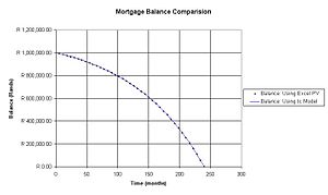 Figure 1
Noting that the balance due P(t) on a loan t years after its inception is simply the present value of the contributions for the remaining period (i.e. T − t), we determine:
The graph(s) in the diagram are a comparison of balance due on a mortgage (1 million for 20 years @ r = 10%) calculated firstly according to the above time continuous model and secondly using the Excel PV function. As may be seen the curves are virtually indistinguishable – calculations effected using the model differ from those effected using the Excel PV function by a mere 0.3% (max). The data from which the graph(s) were derived can be viewed here. The reader may also experiment with a live version of the mortgage balance graph.
Comparison with similar physical systems
Define the "reverse time" variable z = T − t. (t = 0, z = T and t = T, z = 0). Then:
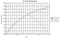 Plotted on a time axis normalized to system time constant (τ = 1/r years and τ = RC seconds respectively) the mortgage balance function in a CRM (green) is a mirror image of the step response curve for an RC circuit (blue).The vertical axis is normalized to system asymptote i.e. perpetuity value Ma/r for the CRM and applied voltage V0 for the RC circuit.
This may be recognized as a solution to the "reverse time" differential equation:
Electrical/electronic engineers and physicists will be familiar with an equation of this nature: it is an exact analogue of the type of differential equation which governs (for example) the charging of a capacitor in an RC circuit.
The key characteristics of such equations are explained in detail at RC circuits. For home owners with mortgages the important parameter to keep in mind is the time constant of the equation which is simply the reciprocal of the annual interest rate r. So (for example) the time constant when the interest rate is 10% is 10 years and the period of a home loan should be determined – within the bounds of affordability – as a minimum multiple of this if the objective is to minimise interest paid on the loan.
Mortgage difference and differential equation
The conventional difference equation for a mortgage loan is relatively straightforward to derive - balance due in each successive period is the previous balance plus per period interest less the per period fixed payment.
Given an annual interest rate r and a borrower with an annual payment capability MN (divided into N equal payments made at time intervals Δt where Δt = 1/N years), we may write:
If N is increased indefinitely so that Δt → 0, we obtain the continuous time differential equation:
Note that for there to be a continually diminishing mortgage balance, the following inequality must hold:
P0 is the same as P(0) – the original loan amount or loan balance at time t = 0.
Solving the difference equation
We begin by re-writing the difference equation in recursive form:
Using the notation Pn to indicate the mortgage balance after n periods, we may apply the recursion relation iteratively to determine P1 and P2:
It can already be seen that the terms containing MN form a geometric series with common ratio 1 + rΔ t. This enables us to write a general expression for Pn:
Finally noting that r Δ t = i the per-period interest rate and MNΔt = x the per period payment, the expression may be written in conventional form:
If the loan timespan is m periods, then Pm = 0 and we obtain the standard present value formula:
Solving the differential equation
One method of solving the equation is to obtain the Laplace transform P(s):
Using a table of Laplace transforms and their time domain equivalents, P(t) may be determined:
In order to fit this solution to the particular start and end points of the mortgage function we need to introduce a time shift of T years (T = loan period) to ensure the function reaches zero at the end of the loan period:
Note that both the original solution and "time-shifted" version satisfy the original differential equation whence both are derived.
Similar to the expression derived above for Pn in the difference equation, the expression for P(t) may be written in the following algebraically equivalent form:
Calculation of accumulated interest and principal payments
Re-arranging the original differential equation we obtain:
Integrating both sides of the equation yields:
The first integral on the right hand side determines the accumulated interest payments from time of inception to time t whilst the second determines the accumulated principal payments over the same period. The sum of these interest and principal payments must equal the cumulative fixed payments at time t i.e. Mat. Evaluating the first integral on the right we obtain an expression for I(t), the interest paid:
Unsurprisingly the second integral evaluates to P0 − P(t) and therefore:
The reader may easily verify that this expression is algebraically identical to the one above.
Loan cost factor
The cost of a loan is simply the annual rate multiplied by loan period:
Let s = rT. Then we may define loan cost factor C(s) such that C = P0C(s) i.e.: C(s) is the cost per unit of currency loaned.
The function C(s) is characterised by having a limiting value of 1 when s is close to zero since for small values of s, exp(−s) ≈ 1 − s and the denominator simplifies to s. Also when s is very large, exp(−s) is small so C(s) ≈ s and thus loan cost C ≈ P0rT (rT >> 0).
By way of example, consider a loan of 1000000 at 10% repaid over 20 years. Then s = 0.1 × 20 = 2.
The product rT is an easily obtained but important parameter in determining loan cost according to the equation C=P0xC(s). This is best illustrated by plotting the cost factor function for s values in domain [0;5]. The resultant graph may be viewed here. The linear behaviour of the function for higher values of s is clear.
Equivalent simple interest cost factor
For a fixed term loan of t years, we may compare the above loan cost factor against an equivalent simple interest cost factor 1+se where se=ret and re is the equivalent simple interest rate:
It is straightforward to determine se in terms of s. Dividing by loan time period t will then give the equivalent simple interest rate. More challenging is the reverse determination of s given se. Submitting the equation to the computational engine at Wolfram Alpha yields the following solution:
where Wn is the Lambert W or product log function.
For example given a loan period of 3 years we may pose the question what interest rate applied to the continuous repayment model yields the same cost factor as a 25% pa simple interest rate applied over the same period. We set se=0.25x3=0.75 and solve for s. The answer divided by 3 gives the continuous repayment equivalent rate as 41.6% pa.
In his book Problem Solving with True Basic,[15] Dr B.D. Hahn has a short section on certain 'hire purchase' schemes in which interest is calculated in advance in one lump sum, which is added to the capital amount, the sum being equally divided over the repayment period. The buyer, however, is often under the impression that the interest is calculated on a reducing balance.
The above example is adapted from the one given in Dr Hahn's book in which he employs the Newton-Raphson algorithm to solve the same problem albeit for a discrete interval (i.e. monthly) repayment loan over the same time period (3 years). As with many similar examples the discrete interval problem and its solution is closely approximated by calculations based on the continuous repayment model - Dr Hahn's solution for interest rate is 40.8% as compared to the 41.6% calculated above.
Period of a loan
If a borrower can afford an annual repayment rate Ma, then we can re-arrange the formula for calculating Ma to obtain an expression for the time period T of a given loan P0:
Minimum Payment Ratio
The minimum payment ratio of a loan is the ratio of minimum possible payment rate to actual payment rate. The minimum possible payment rate is that which just covers the loan interest - a borrower would in theory pay this amount forever because there is never any decrease in loan capital. We will use the letter k to denote minimum payment ratio:
Now we may consider a small re-arrangement of the equation for loan period T:
Plotting s(k) against k gives a very graphic demonstration of why it is a good idea to keep the k value well below the asymptote at k = 1 since in the vicinity thereof, s(k) increases sharply and therefore so does loan cost which is in turn an increasing function of parameter s (rT product).
"Half-life" of a loan
A useful parameter of the mortgage model is the "half-life" of the loan which is the time it takes for the balance on the loan to reach half its original value. To determine the "half-life" we may write:
Solving for t we obtain:
For example applying the formula to some test data (loan of 1 million at 10% for 20 years) we obtain the half-life as 14.34 years. If in practice the loan is being repaid via monthly instalments, the decimal portion can be converted to months and rounded so this answer would equate to 172 months.
Calculation of interest rate
In the discrete time interval model, calculation of a mortgage based interest rate given the remaining parameters has not been possible using analytic methods. Implementations such as the Excel "Rate" function employ a numerical "trial and improvement" method to determine interest rate. At first glance this would also seem to be the case for the continuous repayment model. Given:
we may write:
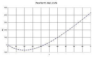 Figure 1
In order to visualise the above as a function of r (for which we wish to determine zeroes), it will be helpful to select numerical values of P0, Ma and T as 10000, 6000 and 3 respectively and plot as shown at right. It will be noted that the function has a minimum value which can be determined by differentiation:
Since the function is approximately parabolic between the roots at r = 0 and the sought value, we may estimate the required root as:
Using this as a starting point, increasingly accurate values for the root may be determined by repeated iterations of the Newton–Raphson algorithm:[17]
Some experimentation on Wolfram Alpha reveals that an exact analytical solution employing the Lambert-W or "product log" function can be obtained. Setting s = MaT/P0 we obtain:
In the region of interest W(−se−s) is a bi-valued function. The first value is just −s which yields the trivial solution r = 0. The second value evaluated within the context of the above formula will provide the required interest rate.
The following table shows calculation of an initial estimate of interest rate followed by a few iterations of the Newton–Raphson algorithm. There is rapid convergence to a solution accurate to several decimal places as may be corroborated against the analytical solution using the Lambert W or "productlog" function on Wolfram Alpha.
Loan (P) Period (T) Annual Payment Rate (Ma) Initial Estimate: 2*Ln(MaT/P)/T 10000 3 6000 39.185778% Newton Raphson Iterations
n r(n) f[r(n)] f'[r(n)] 0 39.185778% -229.57 4444.44 1 44.351111% 21.13 5241.95 2 43.948044% 0.12 5184.06 3 43.945798% 0 5183.74 Present value and future value formulae
Corresponding to the standard formula for the present value of a series of fixed monthly payments, we have already established a time continuous analogue:
In similar fashion, a future value formula can be determined:
In this case the annual rate Ma is determined from a specified (future) savings or sinking fund target PT as follows.
It will be noted that as might be expected:
Another way to calculate balance due P(t) on a continuous-repayment loan is to subtract the future value (at time t) of the payment stream from the future value of the loan (also at time t):
Example
The following example from a school text book[21] will illustrate the conceptual difference between a savings annuity based on discrete time intervals (per month in this case) and one based on continuous payment employing the above future value formula:
On his 30th birthday, an investor decides he wants to accumulate R500000 by his 40th birthday. Starting in one month's time he decides to make equal monthly payments into an account that pays interest at 12% per annum compounded monthly. What monthly payments will he have to make?
For the sake of brevity, we will solve the "discrete interval" problem using the Excel PMT function:
- x(12) = PMT(1%,120,500000) = 2173.55
The amount paid annually would therefore be 26082.57.
For a theoretical continuous payment savings annuity we can only calculate an annual rate of payment:
At this point there is a temptation to simply divide by 12 to obtain a monthly payment. However this would contradict the primary assumption upon which the "continuous payment" model is based: namely that the annual payment rate is defined as:
Since it is of course impossible for an investor to make an infinitely small payment infinite times per annum, a bank or other lending institution wishing to offer "continuous payment" annuities or mortgages would in practice have to choose a large but finite value of N (annual frequency of payments) such that the continuous time formula will always be correct to within some minimal pre-specified error margin. For example hourly fixed payments (calculated using the conventional formula) in this example would accumulate to an annual payment of 25861.07 and the error would be < 0.02%. If the error margin is acceptable, the hourly payment rate can be more simply determined by dividing Ma by 365×24. The (hypothetical) lending institution would then need to ensure its computational resources are sufficient to implement (when required) hourly deductions from customer accounts. In short cash "flow" for continuous payment annuities is to be understood in the very literal sense of the word.
- "Monies paid into a fund in the financial world are paid at discrete – usually equally spaced – points in calendar time. In the continuous process the payment is made continuously, as one might pour fluid from one container into another, where the rate of payment is the fundamental quantity".[22]
The following table shows how as N (annual compounding frequency) increases, the annual payment approaches the limiting value of Ma, the annual payment rate. The difference (error) between annual payment and the limiting value is calculated and expressed as a percentage of the limiting value.
Compounding Period Frequency (N) Per period interest rate Per period payment x(N) Annual Payment % Error Bi-annual 2 6.000000% 13,592.28 27,184.56 5.118918% Quarterly 4 3.000000% 6,631.19 26,524.76 2.567558% Monthly 12 1.000000% 2,173.55 26,082.57 0.857683% Daily 365 0.032877% 70.87 25,868.07 0.028227% Hourly 8760 0.001370% 2.95 25,861.07 0.001176% It will be apparent from the above that the concept of a "continuous repayment" mortgage is a somewhat theoretical construct. Whether it has practical value or not is a question that would need to be carefully considered by economists and actuaries. In particular the meaning of an annual repayment rate must be clearly understood as illustrated in the above example.
However the "continuous payment" model does provide some meaningful insights into the behaviour of the discrete mortgage balance function – in particular that it is largely governed by a time constant equal to the reciprocal of r the nominal annual interest rate. And if a mortgage were to be paid off via fixed daily amounts, then balance due calculations effected using the model would – in general – be accurate to within a small fraction of a percent. Finally the model demonstrates that it is to the modest advantage of the mortgage holder to increase frequency of payment where practically possible.
Summary of formulae and online calculators
Annual payment rate (mortgage loan):

Annual payment rate (sinking fund):

Universal mortgage caculator. Given any three of four variables, this calculates the fourth (unknown) value.
Mortgage Graph. This illustrates the characteristic curve of mortgage balance vs time over a given loan timespan. Loan amount and loan interest rate (p/a) may also be specified. A discrete interval loan will have a very similar characteristic.
Notes
- ^ James, Robert C; James, Glen (1992). Mathematics Dictionary. Chapman and Hall. http://books.google.com/books?id=UyIfgBIwLMQC. - Entry on continuous annuity
- ^ Mathematics Dictionary p.86
- ^ Summation is effected using the standard formula for summation of a geometric sequence.
- ^ An illustration of the summation of terms for a series of 10 annual payments of 10000 at 10% interest can be viewed here.
- ^ Strictly speaking compounding occurs momentarily before payment is deducted so that interest is calculated on the balance as it was before deduction of the period payment.
- ^ Beckwith p. 116: "Technically speaking, the underlying equation is known as an ordinary, linear, first order, inhomogenous, scalar differential equation with a boundary condition."
- ^ Beckwith p.115
- ^ Munem and Foulis p.273
- ^ Beckwith: Equation (29) p. 123.
- ^ See also: Wisdom, John C; Hasselback, James R. (2008). U.S. Master Accounting Guide 2008.. C C H Inc 2008.. http://books.google.com/books?id=l1_FbS0Gj9EC. ps. 470–471
- ^ Beckwith: Equation (31) p. 124.
- ^ Beckwith: Equation (25) p. 123
- ^ Hackman: Equation (2) p.1
- ^ Where equality holds, the mortgage becomes a perpetuity.
- ^ Hahn p. 247
- ^ Beckwith: Equation (23) p. 122. Beckwith uses this formula in relation to a sinking fund but notes (p.124) that the formula is identical for an amortization process.
- ^ Beckwith: (p.125):"In the determination of rates of interest for given continuous payment schedules, it is frequently necessary to determine the roots of transcendental functions.". Beckwith details two methods: Successive substitution and Newton–Raphson. (ps. 126–127).
- ^ See also: King, George (1898). The Theory of Finance. Being a Short Treatise on the Doctrine of Interest and Annuities-Certain. London: Charles and Edwin Layton. Reprinted March 2010 Nabu Press. ISBN 1146318707. http://books.google.com/books?id=ZOWCNpT2cL4C. p. 22. Older actuarial textbooks refer to "interest convertible momently" and "payments momently" when discussing continuous annuities.
- ^ Beckwith: Equation (19) p. 121.
- ^ Beckwith: Equation (27) p. 123.
- ^ Glencross p. 67
- ^ Beckwith p. 114.
- ^ Further worked examples and problems with solutions can be found in Professor Hackman's course notes. See Reference Section.
- ^ Beckwith (pages 128–129) provides more complex examples involving interest rate calculation. The interested reader may verify the calculations by entering the resultant transcendental equations on Wolfram Alpha. Note: the line of working before eqn (38) in Beckwith's article is missing a pair of brackets
References
- Beckwith, R.E. (June 1968). "Continuous Financial Processes". The Journal of Financial and Quantitative Analysis 3 (2): 113–133. JSTOR 2329786.
- Georgia Institute of Technology; Hackman, Steve. "Financial Engineering: ISyE 4803A Course Notes". Georgia Institute of Technology. http://www2.isye.gatech.edu/people/faculty/Steven_Hackman/isye4803E_F08/FixedRateMortgages.pdf. Retrieved 2009-04-27.
- Glencross, M.J. (2007). Mathematics: Grade 12 OBE. Effective Teaching Publishers, Cape Town, RSA.. ISBN 9781920116361.
- Munem, M.A.; Foulis D.J. (1986). Algebra and Trigonometry with Applications.. Worth Publishers, USA.. ISBN 0879012811. http://books.google.co.za/books?id=1cOyXr0W6XIC.
- Hahn, Brian D. (1989). Problem Solving with True Basic.. Juta & Company Limited, Cape Town, South Africa.. ISBN 0702122823. http://books.google.co.za/books?id=OQDhAAAACAAJ&dq.
Bibliography
- Kreyszig, Erwin, Advanced Engineering Mathematics (1998, Wiley Publishers, USA), ISBN 0471154962.
Categories: -
![P_0(1+i)^{n} = \sum_{k=1}^n x(1+i)^{n-k}=\frac{x[(1+i)^n - 1]}{i}](5/b85f787cf822093222c9263c15c25843.png)


![\begin{align}
P_{t+\Delta t} & = P_t+(rP_t-M_N)\Delta t\\[12pt]
\dfrac{P_{t+\Delta t}-P_t}{\Delta t} & = rP_t-M_N
\end{align}](a/27a5f8868569080dbe46cbaa09e2fcb4.png)


-M_N\Delta t\\
&= P_0(1+r\Delta t)^2 - M_N\Delta t(1+r\Delta t)-M_N\Delta t
\end{align}](1/fe11c1875804a53551430ae14dd8e077.png)
![\begin{align}
P_n&=P_0(1+r\Delta t)^n-\sum_{k=1}^{n} M_N\Delta t(1+r\Delta t)^{n-k} \\
&=P_0(1+r\Delta t)^n-\dfrac{M_N\Delta t[(1+r\Delta t)^n - 1]}{r\Delta t}
\end{align}](4/cf4a3c390935f975154257e9ef0e8041.png)
![P_n=P_0(1+i)^n-\dfrac{x[(1+i)^n - 1]}{i}](d/b1df9cb7dfff1aeafa7e01ac35afc670.png)
![P_0=\dfrac{x[1-(1+i)^{-m}]}{i}](1/231222fda3dbc642015d7d226b58e348.png)


![\begin{align}
& P(t) = \frac{M_a}{r}(1-e^{r(t-T)}) \\[8pt]
& P_0 = \frac{M_a}{r}(1-e^{-rT})\Rightarrow\frac{M_a}{r}=\frac{P_0}{1-e^{-rT}} \\[8pt]
\Rightarrow & P(t) = \frac{P_0(1-e^{-r(T-t)})}{1-e^{-rT}}
\end{align}](7/3a7ad3ad0d5aa10b9161ebc5e3c4f7ba.png)


![\begin{align}
& M_a = \frac{P_0 r}{1-e^{-rT}} \\[8pt]
\Rightarrow & T = \frac{1}{r}\ln\frac{M_a}{M_a-P_0 r} = -\frac{1}{r}\ln\left(1 - \frac{P_0 r}{M_a} \right)
\end{align}](5/5e5c5a09211662d3949fd7ddf2808ffa.png)


Wikimedia Foundation. 2010.