- Euler spiral
-
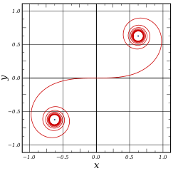 A double-end Euler spiral.
An Euler spiral is a curve whose curvature changes linearly with its curve length (the curvature of a circular curve is equal to the reciprocal of the radius). Euler spirals are also commonly referred to as spiros, clothoids or Cornu spirals.
Euler spirals have applications to diffraction computations. They are also widely used as transition curve in railroad engineering/highway engineering for connecting and transiting the geometry between a tangent and a circular curve. The principle of linear variation of the curvature of the transition curve between a tangent and a circular curve defines the geometry of the Euler spiral:
- Its curvature begins with zero at the straight section (the tangent) and increases linearly with its curve length.
- Where the Euler spiral meets the circular curve, its curvature becomes equal to that of the latter.
Contents
Applications
Track transition curve
Main article: Track transition curveAn object traveling on a circular path experiences a centripetal acceleration. When a vehicle traveling on a straight path approaches a circular path, it experiences a sudden centripetal acceleration starting at the tangent point; and thus centripetal force acts instantly causing much discomfort.
On early railroads this instant application of lateral force was not an issue since low speeds and wide-radius curves were employed (lateral forces on the passengers and the lateral sway was small and tolerable). As speeds of rail vehicles increased over the years, it became obvious that an easement is necessary so that the centripetal acceleration increases linearly with the traveled distance. Given the expression of centripetal acceleration V² / R, the obvious solution is to provide an easement curve whose curvature, 1 / R, increases linearly with the traveled distance. This geometry is an Euler spiral.
Unaware of the solution of the geometry by Leonhard Euler, Rankine cited the cubic curve (a polynomial curve of degree 3), which is an approximation of the Euler spiral for small angular changes in the same way that a parabola is an approximation to a circular curve.
Marie Alfred Cornu (and later some civil engineers) also solved the calculus of Euler spiral independently. Euler spirals are now widely used in rail and highway engineering for providing a transition or an easement between a tangent and a horizontal circular curve.
Optics
The Cornu spiral can be used to describe a diffraction pattern.[1]
Formulation
Symbols

Radius of curvature 
Radius of Circular curve at the end of the spiral 
Angle of curve from beginning of spiral (infinite R) to a particular point on the spiral. This can also be measured as the angle between the initial tangent and the tangent at the concerned point. 
Angle of full spiral curve 
Length measured along the spiral curve from its initial position 
Length of spiral curve Derivation
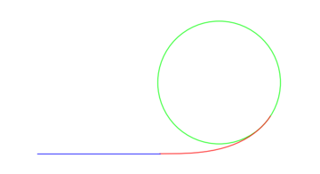
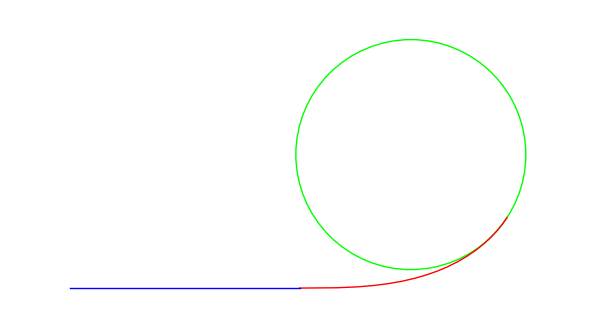
The graph on the right illustrates an Euler spiral used as an easement (transition) curve between two given curves, in this case a straight line (the negative x axis) and a circle. The spiral starts at the origin in the positive x direction and gradually turns anticlockwise to osculate the circle.
The spiral is a small segment of the above double-end Euler spiral in the first quadrant.
- From the definition of the curvature,
- i.e.
- We write in the format,
- Where
- Or
- Thus
- Now
- If
- Then
- Thus
Expansion of Fresnel integral
Main article: Fresnel integralIf a = 1, which is the case for normalized Euler curve, then the Cartesian coordinates are given by Fresnel integrals (or Euler integrals):
Expand C(L) according to power series expansion of cosine:
Expand S(L) according to power series expansion of sine:
Normalization and conclusion
For a given Euler curve with:
or
then
where
 and
and  .
.The process of obtaining solution of (x, y) of an Euler spiral can thus be described as:
- Map L of the original Euler spiral by multiplying with factor a to L' of the normalized Euler spiral;
- Find (x′, y′) from the Fresnel integrals; and
- Map (x′, y′) to (x, y) by scaling up (denormalize) with factor 1 / a. Note that 1 / a > 1.
In the normalization process,
Then
Generally the normalization reduces L' to a small value (<1) and results in good converging characteristics of the Fresnel integral manageable with only a few terms (at a price of increased numerical instability of the calculation, esp. for bigger
values.).Illustration
Given:
Then
And
We scale down the Euler spiral by √60,000, i.e.100√6 to normalized Euler spiral that has:
And
The two angles
are the same. This thus confirm that the original and normalized Euler spirals are having geometric similarity. The locus of the normalized curve can be determined from Fresnel Integral, while the locus of the original Euler spiral can be obtained by scaling back / up or denormalizing.Other properties of normalized Euler spiral
Normalized Euler spiral can be expressed as:
Normalized Euler spiral has the following properties:
And
Note that 2RcLs = 1 also means 1 / Rc = 2Ls, in agreement with the last mathematical statement.
Code for producing an Euler spiral
The following Sage code produces the second graph above. The first four lines express the Euler spiral component. Fresnel functions could not be found. Instead, the integrals of two expanded Taylor series are adopted. The remaining code expresses respectively the tangent and the circle, including the computation for the center coordinates.
  var('L')
  p = integral(taylor(cos(L^2), L, 0, 12), L)
  q = integral(taylor(sin(L^2), L, 0, 12), L)
  r1 = parametric_plot([p, q], (L, 0, 1), color = 'red')

  r2 = line([(-1.0, 0), (0,0)], rgbcolor = 'blue')

  x1 = p.subs(L = 1)
  y1 = q.subs(L = 1)
  R = 0.5
  x2 = x1 - R*sin(1.0)
  y2 = y1 + R*cos(1.0)
  r3 = circle((x2, y2), R, rgbcolor = 'green')
  show(r1 + r2 + r3, aspect_ratio = 1, axes=false)
The following is Mathematica code for the Euler spiral component (it works directly in wolframalpha.com):
  ParametricPlot[
   {FresnelC[Sqrt[2/\[Pi]] t]/Sqrt[2/\[Pi]],
    FresnelS[Sqrt[2/\[Pi]] t]/Sqrt[2/\[Pi]]},
   {t, -10, 10}]
See also
- Fresnel integral
- Geometric design of roads
- Track transition curve
References
- Kellogg, Norman Benjamin (1907). The Transition Curve or Curve of Adjustment (3rd edition ed.). New York: McGraw. http://books.google.com/books?id=ZVZCzW2codgC.
- Weisstein, Eric W., "Cornu Spiral" from MathWorld.
- R. Nave, The Cornu spiral, Hyperphysics (2002) (Uses πt²/2 instead of t².)
- Milton Abramowitz and Irene A. Stegun, eds. Handbook of Mathematical Functions with Formulas, Graphs, and Mathematical Tables. New York: Dover, 1972. (See Chapter 7)
- "Roller Coaster Loop Shapes". http://physics.gu.se/LISEBERG/eng/loop_pe.html. Retrieved 2010-11-12.
External links
Categories:


![\begin{align}
x & = \int_0^L \cos\theta \, ds \\
& = \int_0^L \cos \left[ (a s)^2 \right] ds
\end{align}](f/62f0f13091656cac11368ab0e6c61810.png)


![\begin{align}
y & = \int_0^L \sin\theta \, ds \\
& = \int_0^L \sin \left[ (a s)^2 \right] ds \\
& = \frac{1}{a} \int_0^{L'} \sin {s}^2 \, ds
\end{align}](d/03d8a81c65ea42d4efef6ade90d6de10.png)


Wikimedia Foundation. 2010.