- Pearson's chi-squared test
-
Pearson's chi-squared test (χ2) is the best-known of several chi-squared tests – statistical procedures whose results are evaluated by reference to the chi-squared distribution. Its properties were first investigated by Karl Pearson in 1900.[1] In contexts where it is important to make a distinction between the test statistic and its distribution, names similar to Pearson Χ-squared test or statistic are used.
It tests a null hypothesis stating that the frequency distribution of certain events observed in a sample is consistent with a particular theoretical distribution. The events considered must be mutually exclusive and have total probability 1. A common case for this is where the events each cover an outcome of a categorical variable. A simple example is the hypothesis that an ordinary six-sided die is "fair", i.e., all six outcomes are equally likely to occur.
Contents
Definition
Pearson's chi-squared is used to assess two types of comparison: tests of goodness of fit and tests of independence.
- A test of goodness of fit establishes whether or not an observed frequency distribution differs from a theoretical distribution.
- A test of independence assesses whether paired observations on two variables, expressed in a contingency table, are independent of each other—for example, whether people from different regions differ in the frequency with which they report that they support a political candidate.
The first step in the chi-squared test is to calculate the chi-squared statistic. In order to avoid ambiguity, the value of the test-statistic is denoted by Χ2 rather than χ2 (which is either an uppercase chi instead of lowercase, or an upper case roman X); this also serves as a reminder that the distribution of the test statistic is not exactly that of a chi-squared random variable. However some authors do use the χ2 notation for the test statistic. An exact test which does not rely on using the approximate χ2 distribution is Fisher's exact test: this is substantially more accurate in evaluating the significance level of the test, especially with small numbers of observations.
The chi-squared statistic is calculated by finding the difference between each observed and theoretical frequency for each possible outcome, squaring them, dividing each by the theoretical frequency, and taking the sum of the results. A second important part of determining the test statistic is to define the degrees of freedom of the test: this is essentially the number of observed frequencies adjusted for the effect of using some of those observations to define the theoretical frequencies.
Test for fit of a distribution
Discrete uniform distribution
In this case N observations are divided among n cells. A simple application is to test the hypothesis that, in the general population, values would occur in each cell with equal frequency. The "theoretical frequency" for any cell (under the null hypothesis of a discrete uniform distribution) is thus calculated as
and the reduction in the degrees of freedom is p = 1, notionally because the observed frequencies Oi are constrained to sum to N.
Other distributions
When testing whether observations are random variables whose distribution belongs to a given family of distributions, the "theoretical frequencies" are calculated using a distribution from that family fitted in some standard way. The reduction in the degrees of freedom is calculated as p = s + 1, where s is the number of parameters used in fitting the distribution. For instance, when checking a 3-parameter Weibull distribution, p = 4, and when checking a normal distribution (where the parameters are mean and standard deviation), p = 3. In other words, there will be n − p degrees of freedom, where n is the number of categories.
It should be noted that the degrees of freedom are not based on the number of observations as with a Student's t or F-distribution. For example, if testing for a fair, six-sided die, there would be five degrees of freedom because there are six categories/parameters (each number). The number of times the die is rolled will have absolutely no effect on the number of degrees of freedom.
Calculating the test-statistic
The value of the test-statistic is
where
- Χ2 = Pearson's cumulative test statistic, which asymptotically approaches a χ2 distribution.
- Oi = an observed frequency;
- Ei = an expected (theoretical) frequency, asserted by the null hypothesis;
- n = the number of cells in the table.
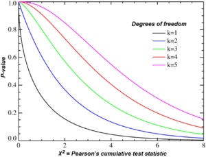 Chi-squared distribution, showing X2 on the x-axis and P-value on the y-axis.
The chi-squared statistic can then be used to calculate a p-value by comparing the value of the statistic to a chi-squared distribution. The number of degrees of freedom is equal to the number of cells n, minus the reduction in degrees of freedom, p.
The result about the number of degrees of freedom is valid when the original data was multinomial and hence the estimated parameters are efficient for minimizing the chi-squared statistic. More generally however, when maximum likelihood estimation does not coincide with minimum chi-squared estimation, the distribution will lie somewhere between a chi-squared distribution with n − 1 − p and n − 1 degrees of freedom (See for instance Chernoff and Lehmann, 1954).
Bayesian method
For more details on this topic, see Categorical distribution#Bayesian statistics.In Bayesian statistics, one would instead use a Dirichlet distribution as conjugate prior. If one took a uniform prior, then the maximum likelihood estimate for the population probability is the observed probability, and one may compute a credible region around this or another estimate.
Test of independence
In this case, an "observation" consists of the values of two outcomes and the null hypothesis is that the occurrence of these outcomes is statistically independent. Each observation is allocated to one cell of a two-dimensional array of cells (called a table) according to the values of the two outcomes. If there are r rows and c columns in the table, the "theoretical frequency" for a cell, given the hypothesis of independence, is
where N is the total sample size (the sum of all cells in the table). The value of the test-statistic is
Fitting the model of "independence" reduces the number of degrees of freedom by p = r + c − 1. The number of degrees of freedom is equal to the number of cells rc, minus the reduction in degrees of freedom, p, which reduces to (r − 1)(c − 1).
For the test of independence, a chi-squared probability of less than or equal to 0.05 (or the chi-squared statistic being at or larger than the 0.05 critical point) is commonly interpreted by applied workers as justification for rejecting the null hypothesis that the row variable is independent of the column variable.[2] The alternative hypothesis corresponds to the variables having an association or relationship where the structure of this relationship is not specified.
Assumptions
The chi-squared test, when used with the standard approximation that a chi-squared distribution is applicable, has the following assumptions:[citation needed]
- Simple random sample – The sample data is a random sampling from a fixed distribution or population where each member of the population has an equal probability of selection. Variants of the test have been developed for complex samples, such as where the data is weighted.
- Sample size (whole table) – A sample with a sufficiently large size is assumed. If a chi squared test is conducted on a sample with a smaller size, then the chi squared test will yield an inaccurate inference. The researcher, by using chi squared test on small samples, might end up committing a Type II error.
- Expected cell count – Adequate expected cell counts. Some require 5 or more, and others require 10 or more. A common rule is 5 or more in all cells of a 2-by-2 table, and 5 or more in 80% of cells in larger tables, but no cells with zero expected count. When this assumption is not met, Yates's correction is applied.
- Independence – The observations are always assumed to be independent of each other. This means chi-squared cannot be used to test correlated data (like matched pairs or panel data). In those cases you might want to turn to McNemar's test.
Examples
Goodness of fit
For example, to test the hypothesis that a random sample of 100 people has been drawn from a population in which men and women are equal in frequency, the observed number of men and women would be compared to the theoretical frequencies of 50 men and 50 women. If there were 44 men in the sample and 56 women, then
If the null hypothesis is true (i.e., men and women are chosen with equal probability in the sample), the test statistic will be drawn from a chi-squared distribution with one degree of freedom. Though one might expect two degrees of freedom (one each for the men and women), we must take into account that the total number of men and women is constrained (100), and thus there is only one degree of freedom (2 − 1). Alternatively, if the male count is known the female count is determined, and vice-versa.
Consultation of the chi-squared distribution for 1 degree of freedom shows that the probability of observing this difference (or a more extreme difference than this) if men and women are equally numerous in the population is approximately 0.23. This probability is higher than conventional criteria for statistical significance (.001-.05), so normally we would not reject the null hypothesis that the number of men in the population is the same as the number of women (i.e. we would consider our sample within the range of what we'd expect for a 50/50 male/female ratio.)
Problems
The approximation to the chi-squared distribution breaks down if expected frequencies are too low. It will normally be acceptable so long as no more than 20% of the events have expected frequencies below 5. Where there is only 1 degree of freedom, the approximation is not reliable if expected frequencies are below 10. In this case, a better approximation can be obtained by reducing the absolute value of each difference between observed and expected frequencies by 0.5 before squaring; this is called Yates's correction for continuity.
In cases where the expected value, E, is found to be small (indicating either a small underlying population probability, or a small number of observations), the normal approximation of the multinomial distribution can fail, and in such cases it is found to be more appropriate to use the G-test, a likelihood ratio-based test statistic. Where the total sample size is small, it is necessary to use an appropriate exact test, typically either the binomial test or (for contingency tables) Fisher's exact test; but note that this test assumes fixed and known marginal totals.
Distribution
The null distribution of the Pearson statistic with j rows and k columns is approximated by the chi-squared distribution with (k − 1)(j − 1) degrees of freedom.[3]
This approximation arises as the true distribution, under the null hypothesis, if the expected value is given by a multinomial distribution. For large sample sizes, the central limit theorem says this distribution tends toward a certain multivariate normal distribution.
Two cells
In the special case where there are only two cells in the table, the expected values follow a binomial distribution,
where
- p = probability, under the null hypothesis,
- n = number of observations in the sample.
In the above example the hypothesised probability of a male observation is 0.5, with 100 samples. Thus we expect to observe 50 males.
If n is sufficiently large, the above binomial distribution may be approximated by a Gaussian (normal) distribution and thus the Pearson test statistic approximates a chi-squared distribution,
Let O1 be the number of observations from the sample that are in the first cell. The Pearson test statistic can be expressed as
which can in turn be expressed as
By the normal approximation to a binomial this is the squared of one standard normal variate, and hence is distributed as chi-squared with 1 degree of freedom. Note that the denominator is one standard deviation of the Gaussian approximation, so can be written
So as consistent with the meaning of the chi-squared distribution, we are measuring how probable the observed number of standard deviations away from the mean is under the Gaussian approximation (which is a good approximation for large n).
The chi-squared distribution is then integrated on the right of the statistic value to obtain the P-value, which is equal to the probability of getting a statistic equal or bigger than the observed one, assuming the null hypothesis.
Two-by-two contingency tables
When the test is applied to a contingency table containing two rows and two columns, the test is equivalent to a Z-test of proportions.
Many cells
Similar arguments as above lead to the desired result.[citation needed] Each cell (except the final one, whose value is completely determined by the others) is treated as an independent binomial variable, and their contributions are summed and each contributes one degree of freedom.
See also
- Degrees of freedom (statistics), including Degrees of freedom (statistics)#Effective degrees of freedom for correlated observations and regularized models
- Fisher's exact test
- Median test
- Chi-squared test
- Chi-squared nomogram
- Deviance (statistics), another measure of the quality of fit.
- Yates's correction for continuity
- Mann–Whitney U
- Cramér's V - a measure of correlation for the chi-squared test.
Notes
- ^ Karl Pearson (1900). "On the criterion that a given system of deviations from the probable in the case of a correlated system of variables is such that it can be reasonably supposed to have arisen from random sampling". Philosophical Magazine, Series 5 50 (302): 157–175. doi:10.1080/14786440009463897.
- ^ "Critical Values of the Chi-Squared Distribution". NIST/SEMATECH e-Handbook of Statistical Methods. National Institute of Standards and Technology. http://www.itl.nist.gov/div898/handbook/eda/section3/eda3674.htm.
- ^ Statistics for Applications. MIT OpenCourseWare. Lecture 23. Pearson's Theorem. Retrieved 21 March 2007.
References
- Chernoff, H.; Lehmann E.L. (1954). "The use of maximum likelihood estimates in χ2 tests for goodness-of-fit". The Annals of Mathematical Statistics 25 (3): 579–586. doi:10.1214/aoms/1177728726.
- Plackett, R.L. (1983). "Karl Pearson and the Chi-Squared Test". International Statistical Review (International Statistical Institute (ISI)) 51 (1): 59–72. doi:10.2307/1402731. JSTOR 1402731.
- Greenwood, P.E., Nikulin, M.S.(1996). A guide to chi-squared testing, J.Wiley, New York, ISBN 0-471-55779-X.
External links
- A video comparison of Chi-Squared Fitting Engines in Excel
- Chi-squared tests of contingency tables
- Chi-Squared Applet Calculator
- Sampling Distribution of the Sample Chi-Squared Statistic — a Java applet showing the sampling distribution of the Pearson test statistic.
- Online Chi-Squared Test for uniform distribution
- Chi-Squared distribution table
- A tutorial on the chi-squared test devised for Oxford University psychology students
Categories:- Categorical data
- Normality tests
- Statistical tests
- Statistical approximations


Wikimedia Foundation. 2010.