- Principal component analysis
-
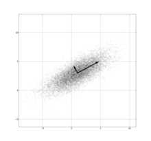 PCA of a multivariate Gaussian distribution centered at (1,3) with a standard deviation of 3 in roughly the (0.878, 0.478) direction and of 1 in the orthogonal direction. The vectors shown are the eigenvectors of the covariance matrix scaled by the square root of the corresponding eigenvalue, and shifted so their tails are at the mean.
Principal component analysis (PCA) is a mathematical procedure that uses an orthogonal transformation to convert a set of observations of possibly correlated variables into a set of values of uncorrelated variables called principal components. The number of principal components is less than or equal to the number of original variables. This transformation is defined in such a way that the first principal component has as high a variance as possible (that is, accounts for as much of the variability in the data as possible), and each succeeding component in turn has the highest variance possible under the constraint that it be orthogonal to (uncorrelated with) the preceding components. Principal components are guaranteed to be independent only if the data set is jointly normally distributed. PCA is sensitive to the relative scaling of the original variables. Depending on the field of application, it is also named the discrete Karhunen–Loève transform (KLT), the Hotelling transform or proper orthogonal decomposition (POD).
PCA was invented in 1901 by Karl Pearson.[1] Now it is mostly used as a tool in exploratory data analysis and for making predictive models. PCA can be done by eigenvalue decomposition of a data covariance matrix or singular value decomposition of a data matrix, usually after mean centering the data for each attribute. The results of a PCA are usually discussed in terms of component scores (the transformed variable values corresponding to a particular case in the data) and loadings (the weight by which each standardized original variable should be multiplied to get the component score).[2]
PCA is the simplest of the true eigenvector-based multivariate analyses. Often, its operation can be thought of as revealing the internal structure of the data in a way which best explains the variance in the data. If a multivariate dataset is visualised as a set of coordinates in a high-dimensional data space (1 axis per variable), PCA can supply the user with a lower-dimensional picture, a "shadow" of this object when viewed from its (in some sense) most informative viewpoint. This is done by using only the first few principal components so that the dimensionality of the transformed data is reduced.
PCA is closely related to factor analysis; indeed, some statistical packages deliberately conflate the two techniques. True factor analysis makes different assumptions about the underlying structure and solves eigenvectors of a slightly different matrix.
Details
PCA is mathematically defined[3] as an orthogonal linear transformation that transforms the data to a new coordinate system such that the greatest variance by any projection of the data comes to lie on the first coordinate (called the first principal component), the second greatest variance on the second coordinate, and so on.
Define a data matrix, XT, with zero empirical mean (the empirical (sample) mean of the distribution has been subtracted from the data set), where each of the n rows represents a different repetition of the experiment, and each of the m columns gives a particular kind of datum (say, the results from a particular probe). (Note that what we are calling XT is often alternatively denoted as X itself.) The singular value decomposition of X is X = WΣVT, where the m × m matrix W is the matrix of eigenvectors of XXT, the matrix Σ is an m × n rectangular diagonal matrix with nonnegative real numbers on the diagonal, and the n × n matrix V is the matrix of eigenvectors of XTX. The PCA transformation that preserves dimensionality (that is, gives the same number of principal components as original variables) is then given by:
V is not uniquely defined in the usual case when m < n − 1, but Y will usually still be uniquely defined. Since W (by definition of the SVD of a real matrix) is an orthogonal matrix, each row of YT is simply a rotation of the corresponding row of XT. The first column of YT is made up of the "scores" of the cases with respect to the "principal" component, the next column has the scores with respect to the "second principal" component, and so on.
If we want a reduced-dimensionality representation, we can project X down into the reduced space defined by only the first L singular vectors, WL:
 where
where  with
with  the
the  rectangular identity matrix.
The matrix W of singular vectors of X is equivalently the matrix W of eigenvectors of the matrix of observed covariances C = X XT,
Given a set of points in Euclidean space, the first principal component corresponds to a line that passes through the multidimensional mean and minimizes the sum of squares of the distances of the points from the line. The second principal component corresponds to the same concept after all correlation with the first principal component has been subtracted from the points. The singular values (in Σ) are the square roots of the eigenvalues of the matrix XXT. Each eigenvalue is proportional to the portion of the "variance" (more correctly of the sum of the squared distances of the points from their multidimensional mean) that is correlated with each eigenvector. The sum of all the eigenvalues is equal to the sum of the squared distances of the points from their multidimensional mean. PCA essentially rotates the set of points around their mean in order to align with the principal components. This moves as much of the variance as possible (using an orthogonal transformation) into the first few dimensions. The values in the remaining dimensions, therefore, tend to be small and may be dropped with minimal loss of information. PCA is often used in this manner for dimensionality reduction. PCA has the distinction of being the optimal orthogonal transformation for keeping the subspace that has largest "variance" (as defined above). This advantage, however, comes at the price of greater computational requirements if compared, for example and when applicable, to the discrete cosine transform. Nonlinear dimensionality reduction techniques tend to be more computationally demanding than PCA.
PCA is sensitive to the scaling of the variables. If we have just two variables and they have the same sample variance and are positively correlated, then the PCA will entail a rotation by 45° and the "loadings" for the two variables with respect to the principal component will be equal. But if we multiply all values of the first variable by 100, then the principal component will be almost the same as that variable, with a small contribution from the other variable, whereas the second component will be almost aligned with the second original variable. This means that whenever the different variables have different units (like temperature and mass), PCA is a somewhat arbitrary method of analysis. (Different results would be obtained if one used Fahrenheit rather than Celsius for example.) Note that Pearson's original paper was entitled "On Lines and Planes of Closest Fit to Systems of Points in Space" – "in space" implies physical Euclidean space where such concerns do not arise. One way of making the PCA less arbitrary is to use variables scaled so as to have unit variance.
Discussion
Mean subtraction (a.k.a. "mean centering") is necessary for performing PCA to ensure that the first principal component describes the direction of maximum variance. If mean subtraction is not performed, the first principal component might instead correspond more or less to the mean of the data. A mean of zero is needed for finding a basis that minimizes the mean square error of the approximation of the data.[4]
Assuming zero empirical mean (the empirical mean of the distribution has been subtracted from the data set), the principal component w1 of a data set X can be defined as:
(See arg max for the notation.) With the first k − 1 components, the kth component can be found by subtracting the first k − 1 principal components from X:
and by substituting this as the new data set to find a principal component in
PCA is equivalent to empirical orthogonal functions (EOF), a name which is used in meteorology.
An autoencoder neural network with a linear hidden layer is similar to PCA. Upon convergence, the weight vectors of the K neurons in the hidden layer will form a basis for the space spanned by the first K principal components. Unlike PCA, this technique will not necessarily produce orthogonal vectors.
PCA is a popular primary technique in pattern recognition. It is not, however, optimized for class separability.[5] An alternative is the linear discriminant analysis, which does take this into account.
Table of symbols and abbreviations
Symbol Meaning Dimensions Indices ![\mathbf{X} = \{ X[m,n] \}](5/4f5edaf547b2bccd71d0cf5e87dff571.png)
data matrix, consisting of the set of all data vectors, one vector per column 


the number of column vectors in the data set 
scalar 
the number of elements in each column vector (dimension) scalar 
the number of dimensions in the dimensionally reduced subspace, 
scalar ![\mathbf{u} = \{ u[m] \}](3/243cfa44b5c134ab36cee838370ab10f.png)
vector of empirical means, one mean for each row m of the data matrix 
![\mathbf{s} = \{ s[m] \}](b/62b0f4ebcc25bae3a1483ed6cb5f8a0f.png)
vector of empirical standard deviations, one standard deviation for each row m of the data matrix ![\mathbf{h} = \{ h[n] \}](6/a7633ff205e8e12c57305ae6e6ec6b0d.png)
vector of all 1's 
![\mathbf{B} = \{ B[m,n] \}](f/f0f5973e1e39f5c57d535f61d884a8db.png)
deviations from the mean of each row m of the data matrix
![\mathbf{Z} = \{ Z[m,n] \}](2/742fc32b598a672ddf488380552b9a3e.png)
z-scores, computed using the mean and standard deviation for each row m of the data matrix
![\mathbf{C} = \{ C[p,q] \}](c/09cc2e594024a2d253a92085f2fa971e.png)
covariance matrix 


![\mathbf{R} = \{ R[p,q] \}](1/c112fbe1a768f79a01c450347f31f66d.png)
correlation matrix
![\mathbf{V} = \{ V[p,q] \}](0/cd06867ae466e6cc51b510390a102a30.png)
matrix consisting of the set of all eigenvectors of C, one eigenvector per column
![\mathbf{D} = \{ D[p,q] \}](8/ee81ef7ee451dc3cbcf3be2e27785fe8.png)
diagonal matrix consisting of the set of all eigenvalues of C along its principal diagonal, and 0 for all other elements
![\mathbf{W} = \{ W[p,q] \}](e/9ce17dc9bae96640247f237a83fec8d7.png)
matrix of basis vectors, one vector per column, where each basis vector is one of the eigenvectors of C, and where the vectors in W are a sub-set of those in V 

![\mathbf{Y} = \{ Y[m,n] \}](1/6f10889c51fda552dc6a278ecda60abf.png)
matrix consisting of N column vectors, where each vector is the projection of the corresponding data vector from matrix X onto the basis vectors contained in the columns of matrix W. 

Properties and limitations of PCA
As noted above, the results of PCA depend on the scaling of the variables.
The applicability of PCA is limited by certain assumptions[6] made in its derivation.
Computing PCA using the covariance method
The following is a detailed description of PCA using the covariance method (see also here). But note that it is better to use the singular value decomposition (using standard software).
The goal is to transform a given data set X of dimension M to an alternative data set Y of smaller dimension L. Equivalently, we are seeking to find the matrix Y, where Y is the Karhunen–Loève transform (KLT) of matrix X:
Organize the data set
Suppose you have data comprising a set of observations of M variables, and you want to reduce the data so that each observation can be described with only L variables, L < M. Suppose further, that the data are arranged as a set of N data vectors
 with each
  representing a single grouped observation of the M variables.
- Write as column vectors, each of which has M rows.
- Place the column vectors into a single matrix X of dimensions M × N.
Calculate the empirical mean
- Find the empirical mean along each dimension m = 1, ..., M.
- Place the calculated mean values into an empirical mean vector u of dimensions M × 1.
Calculate the deviations from the mean
Mean subtraction is an integral part of the solution towards finding a principal component basis that minimizes the mean square error of approximating the data.[7] Hence we proceed by centering the data as follows:
- Subtract the empirical mean vector u from each column of the data matrix X.
- Store mean-subtracted data in the M × N matrix B.
-

- where h is a 1 × N row vector of all 1s:
Find the covariance matrix
- Find the M × M empirical covariance matrix C from the outer product of matrix B with itself:
-
![\mathbf{C} = \mathbb{ E } \left[ \mathbf{B} \otimes \mathbf{B} \right] = \mathbb{ E } \left[ \mathbf{B} \cdot \mathbf{B}^{*} \right] = { 1 \over N } \sum_{} \mathbf{B} \cdot \mathbf{B}^{*}](5/065b349b478404457a2c13e42f79ce8c.png)
- where
 is the expected value operator,
 is the outer product operator, and
 is the conjugate transpose operator. Note that if B consists entirely of real numbers, which is the case in many applications, the "conjugate transpose" is the same as the regular transpose.
- Please note that the information in this section is indeed a bit fuzzy. Outer products apply to vectors. For tensor cases we should apply tensor products, but the covariance matrix in PCA is a sum of outer products between its sample vectors; indeed, it could be represented as B.B*. See the covariance matrix sections on the discussion page for more information.
Find the eigenvectors and eigenvalues of the covariance matrix
- Compute the matrix V of eigenvectors which diagonalizes the covariance matrix C:
- where D is the diagonal matrix of eigenvalues of C. This step will typically involve the use of a computer-based algorithm for computing eigenvectors and eigenvalues. These algorithms are readily available as sub-components of most matrix algebra systems, such as R (programming language), MATLAB,[8][9] Mathematica,[10] SciPy, IDL(Interactive Data Language), or GNU Octave as well as OpenCV.
- Matrix D will take the form of an M × M diagonal matrix, where
- is the mth eigenvalue of the covariance matrix C, and
- Matrix V, also of dimension M × M, contains M column vectors, each of length M, which represent the M eigenvectors of the covariance matrix C.
- The eigenvalues and eigenvectors are ordered and paired. The mth eigenvalue corresponds to the mth eigenvector.
Rearrange the eigenvectors and eigenvalues
- Sort the columns of the eigenvector matrix V and eigenvalue matrix D in order of decreasing eigenvalue.
- Make sure to maintain the correct pairings between the columns in each matrix.
Compute the cumulative energy content for each eigenvector
- The eigenvalues represent the distribution of the source data's energy[clarification needed] among each of the eigenvectors, where the eigenvectors form a basis for the data. The cumulative energy content g for the mth eigenvector is the sum of the energy content across all of the eigenvalues from 1 through m:
Select a subset of the eigenvectors as basis vectors
- Save the first L columns of V as the M × L matrix W:
- where
- Use the vector g as a guide in choosing an appropriate value for L. The goal is to choose a value of L as small as possible while achieving a reasonably high value of g on a percentage basis. For example, you may want to choose L so that the cumulative energy g is above a certain threshold, like 90 percent. In this case, choose the smallest value of L such that
Convert the source data to z-scores
- Create an M × 1 empirical standard deviation vector s from the square root of each element along the main diagonal of the covariance matrix C:
- Calculate the M × N z-score matrix:
-
 (divide element-by-element)
- Note: While this step is useful for various applications as it normalizes the data set with respect to its variance, it is not integral part of PCA/KLT
Project the z-scores of the data onto the new basis
- The projected vectors are the columns of the matrix
- W* is the conjugate transpose of the eigenvector matrix.
- The columns of matrix Y represent the Karhunen–Loeve transforms (KLT) of the data vectors in the columns of matrix X.
Derivation of PCA using the covariance method
Let X be a d-dimensional random vector expressed as column vector. Without loss of generality, assume X has zero mean.
We want to find
 a
a  orthonormal transformation matrix P so that PX has a diagonal covariant matrix (i.e. PX is a random vector with all its distinct components pairwise uncorrelated).
A quick computation assuming P were unitary yields:
Hence
holds if and only if  were diagonalisable by P.
This is very constructive, as cov(X) is guaranteed to be a non-negative definite matrix and thus is guaranteed to be diagonalisable by some unitary matrix.
Computing principal components iteratively
In practical implementations especially with high dimensional data (large m), the covariance method is rarely used because it is not efficient. One way to compute the first principal component efficiently[11] is shown in the following pseudo-code, for a data matrix XT with zero mean, without ever computing its covariance matrix. Note that here a zero mean data matrix means that the columns of XT should each have zero mean.
 a random vector
do c times:
a random vector
do c times:
 (a vector of length m)
for each row
(a vector of length m)
for each row 

 return
This algorithm is simply an efficient way of calculating XXTp, normalizing, and placing the result back in p (Power iteration). It avoids the nm2 operations of calculating the covariance matrix. p will typically get close to the first principal component of XT within a small number of iterations, c. (The magnitude of t will be larger after each iteration. Convergence can be detected when it increases by an amount too small for the precision of the machine.)
Subsequent principal components can be computed by subtracting component p from XT (see Gram–Schmidt) and then repeating this algorithm to find the next principal component. However this simple approach is not numerically stable if more than a small number of principal components are required, because imprecisions in the calculations will additively affect the estimates of subsequent principal components. More advanced methods build on this basic idea, as with the closely related Lanczos algorithm.
One way to compute the eigenvalue that corresponds with each principal component is to measure the difference in sum-squared-distance between the rows and the mean, before and after subtracting out the principal component. The eigenvalue that corresponds with the component that was removed is equal to this difference.
The NIPALS method
Main article: Non-linear iterative partial least squaresFor very high-dimensional datasets, such as those generated in the *omics sciences (e.g., genomics, metabolomics) it is usually only necessary to compute the first few PCs. The non-linear iterative partial least squares (NIPALS) algorithm calculates t1 and p1' from X. The outer product, t1p1' can then be subtracted from X leaving the residual matrix E1. This can be then used to calculate subsequent PCs.[12] This results in a dramatic reduction in computational time since calculation of the covariance matrix is avoided.
Relation between PCA and K-means clustering
It has been shown recently (2007)[13][14] that the relaxed solution of K-means clustering, specified by the cluster indicators, is given by the PCA principal components, and the PCA subspace spanned by the principal directions is identical to the cluster centroid subspace specified by the between-class scatter matrix. Thus PCA automatically projects to the subspace where the global solution of K-means clustering lies, and thus facilitates K-means clustering to find near-optimal solutions.
Correspondence analysis
Correspondence analysis (CA) was developed by Jean-Paul Benzécri[15] and is conceptually similar to PCA, but scales the data (which should be non-negative) so that rows and columns are treated equivalently. It is traditionally applied to contingency tables. CA decomposes the chi-squared statistic associated to this table into orthogonal factors.[16] Because CA is a descriptive technique, it can be applied to tables for which the chi-squared statistic is appropriate or not. Several variants of CA are available including detrended correspondence analysis and canonical correspondence analysis. One special extension is multiple correspondence analysis, which may be seen as the counterpart of principal component analysis for categorical data.[17]
Generalizations
Nonlinear generalizations
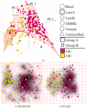 Linear PCA versus nonlinear Principal Manifolds[18] for visualization of breast cancer microarray data: a) Configuration of nodes and 2D Principal Surface in the 3D PCA linear manifold. The dataset is curved and can not be mapped adequately on a 2D principal plane; b) The distribution in the internal 2D non-linear principal surface coordinates (ELMap2D) together with an estimation of the density of points; c) The same as b), but for the linear 2D PCA manifold (PCA2D). The "basal" breast cancer subtype is visualized more adequately with ELMap2D and some features of the distribution become better resolved in comparison to PCA2D. Principal manifolds are produced by the elastic maps algorithm. Data are available for public competition.[19]
Most of the modern methods for nonlinear dimensionality reduction find their theoretical and algorithmic roots in PCA or K-means. Pearson's original idea was to take a straight line (or plane) which will be "the best fit" to a set of data points. Principal curves and manifolds[20] give the natural geometric framework for PCA generalization and extend the geometric interpretation of PCA by explicitly constructing an embedded manifold for data approximation, and by encoding using standard geometric projection onto the manifold, as it is illustrated by Fig. See also the elastic map algorithm and principal geodesic analysis.
Multilinear generalizations
In multilinear subspace learning, PCA is generalized to multilinear PCA (MPCA) that extracts features directly from tensor representations. MPCA is solved by performing PCA in each mode of the tensor iteratively. MPCA has been applied to face recognition, gait recognition, etc. MPCA is further extended to uncorrelated MPCA, non-negative MPCA and robust MPCA.
Higher order
N-way principal component analysis may be performed with models such as Tucker decomposition, PARAFAC, multiple factor analysis, co-inertia analysis, STATIS, and DISTATIS.
Robustness - Weighted PCA
While PCA finds the mathematically optimal method (as in minimizing the squared error), it is sensitive to outliers in the data that produce large errors PCA tries to avoid. It therefore is common practice to remove outliers before computing PCA. However, in some contexts, outliers can be difficult to identify. For example in data mining algorithms like correlation clustering, the assignment of points to clusters and outliers is not known beforehand. A recently proposed generalization of PCA [21] based on a Weighted PCA increases robustness by assigning different weights to data objects based on their estimated relevancy.
Software/source code
- Cornell Spectrum Imager - An open-source toolset built on ImageJ. Enables quick easy PCA analysis for 3D datacubes.
- imDEV Free Excel addin to calculate principal components using R package pcaMethods.
- "ViSta: The Visual Statistics System" a free software that provides principal components analysis, simple and multiple correspondence analysis.
- "Spectramap" is software to create a biplot using principal components analysis, correspondence analysis or spectral map analysis.
- XLSTAT is a statistical and multivariate analysis software including Principal Component Analysis among other multivariate tools.
- FinMath, a .NET numerical library containing an implementation of PCA.
- The Unscrambler is a multivariate analysis software enabling Principal Component Analysis (PCA) with PCA Projection.
- Computer Vision Library
- In the MATLAB Statistics Toolbox, the functions
princompandwmspcagive the principal components, while the functionpcaresgives the residuals and reconstructed matrix for a low-rank PCA approximation. Here is a link to a MATLAB implementation of PCAPcaPress. - NMath, a numerical library containing PCA for the .NET Framework.
- in Octave, a free software computational environment mostly compatible with MATLAB, the function
princompgives the principal component. - in the free statistical package R, the functions
princompandprcompcan be used for principal component analysis;prcompuses singular value decomposition which generally gives better numerical accuracy. Recently there has been an explosion in implementations of principal component analysis in various R packages, generally in packages for specific purposes. For a more complete list, see here: [1]. - In XLMiner, the Principal Components tab can be used for principal component analysis.
- In IDL, the principal components can be calculated using the function
pcomp. - Weka computes principal components (javadoc).
- Software for analyzing multivariate data with instant response using PCA
- Orange (software) supports PCA through its Linear Projection widget.
- A version of PCA adapted for population genetics analysis can be found in the suite EIGENSOFT.
- PCA can also be performed by the statistical software Partek Genomics Suite, developed by Partek.
See also
- Multilinear PCA
- Correspondence analysis
- Eigenface
- Exploratory factor analysis (Wikiversity)
- Geometric data analysis
- Factorial code
- Independent component analysis
- Kernel PCA
- Matrix decomposition
- Nonlinear dimensionality reduction
- Oja's rule
- Point distribution model (PCA applied to morphometry and computer vision)
- Principal component regression
- Principal component analysis (Wikibooks)
- Singular spectrum analysis
- Singular value decomposition
- Sparse PCA
- Transform coding
- Weighted least squares
- Dynamic mode decomposition
Notes
- ^ Pearson, K. (1901). "On Lines and Planes of Closest Fit to Systems of Points in Space" (PDF). Philosophical Magazine 2 (6): 559–572. http://stat.smmu.edu.cn/history/pearson1901.pdf.
- ^ Shaw PJA (2003) Multivariate statistics for the Environmental Sciences, Hodder-Arnold. ISBN 0-3408-0763-6.[page needed]
- ^ Jolliffe I.T. Principal Component Analysis, Series: Springer Series in Statistics, 2nd ed., Springer, NY, 2002, XXIX, 487 p. 28 illus. ISBN 978-0-387-95442-4
- ^ A. A. Miranda, Y. A. Le Borgne, and G. Bontempi. New Routes from Minimal Approximation Error to Principal Components, Volume 27, Number 3 / June, 2008, Neural Processing Letters, Springer
- ^ Fukunaga, Keinosuke (1990). Introduction to Statistical Pattern Recognition. Elsevier. ISBN 0122698517. http://books.google.com/books?visbn=0122698517.
- ^ Jonathon Shlens, A Tutorial on Principal Component Analysis.
- ^ A.A. Miranda, Y.-A. Le Borgne, and G. Bontempi. New Routes from Minimal Approximation Error to Principal Components, Volume 27, Number 3 / June, 2008, Neural Processing Letters, Springer
- ^ eig function Matlab documentation
- ^ MATLAB PCA-based Face recognition software
- ^ Eigenvalues function Mathematica documentation
- ^ Roweis, Sam. "EM Algorithms for PCA and SPCA." Advances in Neural Information Processing Systems. Ed. Michael I. Jordan, Michael J. Kearns, and Sara A. Solla The MIT Press, 1998.
- ^ Geladi, Paul; Kowalski, Bruce (1986). "Partial Least Squares Regression:A Tutorial". Analytica Chimica Acta 185: 1–17. doi:10.1016/0003-2670(86)80028-9.
- ^ H. Zha, C. Ding, M. Gu, X. He and H.D. Simon. "Spectral Relaxation for K-means Clustering", http://ranger.uta.edu/~chqding/papers/Zha-Kmeans.pdf, Neural Information Processing Systems vol.14 (NIPS 2001). pp. 1057–1064, Vancouver, Canada. Dec. 2001.
- ^ C. Ding and X. He. "K-means Clustering via Principal Component Analysis". Proc. of Int'l Conf. Machine Learning (ICML 2004), pp 225–232. July 2004. http://ranger.uta.edu/~chqding/papers/KmeansPCA1.pdf
- ^ Benzécri, J.-P. (1973). L'Analyse des Données. Volume II. L'Analyse des Correspondances. Paris, France: Dunod.
- ^ Greenacre, Michael (1983). Theory and Applications of Correspondence Analysis. London: Academic Press. ISBN 0-12-299050-1.
- ^ Le Roux, Brigitte and Henry Rouanet (2004). Geometric Data Analysis, From Correspondence Analysis to Structured Data Analysis. Dordrecht: Kluwer.
- ^ A. N. Gorban, A. Y. Zinovyev, Principal Graphs and Manifolds, In: Handbook of Research on Machine Learning Applications and Trends: Algorithms, Methods and Techniques, Olivas E.S. et al Eds. Information Science Reference, IGI Global: Hershey, PA, USA, 2009. 28-59.
- ^ Wang, Y., Klijn, J.G., Zhang, Y., Sieuwerts, A.M., Look, M.P., Yang, F., Talantov, D., Timmermans, M., Meijer-van Gelder, M.E., Yu, J. et al.: Gene expression profiles to predict distant metastasis of lymph-node-negative primary breast cancer. Lancet 365, 671-679 (2005); Data online
- ^ A. Gorban, B. Kegl, D. Wunsch, A. Zinovyev (Eds.), Principal Manifolds for Data Visualisation and Dimension Reduction, LNCSE 58, Springer, Berlin – Heidelberg – New York, 2007. ISBN 978-3-540-73749-0
- ^ Kriegel, H. P.; Kröger, P.; Schubert, E.; Zimek, A. (2008). "A General Framework for Increasing the Robustness of PCA-Based Correlation Clustering Algorithms". Scientific and Statistical Database Management. Lecture Notes in Computer Science 5069: 418. doi:10.1007/978-3-540-69497-7_27. ISBN 978-3-540-69476-2.
References
- Jolliffe, I. T. (1986). Principal Component Analysis. Springer-Verlag. pp. 487. doi:10.1007/b98835. ISBN 978-0-387-95442-4. http://www.springer.com/west/home/new+%26+forthcoming+titles+%28default%29?SGWID=4-40356-22-2285433-0.


![u[m] = {1 \over N} \sum_{n=1}^N X[m,n]](5/8957f38829f7b6c873a6248176f16b58.png)
![h[n] = 1 \, \qquad \qquad \text{for } n = 1, \ldots, N](a/2eab23221256ff7f9520579f8fe04a8e.png)

![D[p,q] = \lambda_m \qquad \text{for } p = q = m](8/e88355eb4cb2eb58ab02626b1050400f.png)
![D[p,q] = 0 \qquad \text{for } p \ne q.](c/dac4a5b1fcba2b50e3f18762999149a9.png)
![g[m] = \sum_{q=1}^m D[q,q] \qquad \mathrm{for} \qquad m = 1,\dots,M](9/d197580a393c78139fc14d101901cc62.png) [
[![W[p,q] = V[p,q] \qquad \mathrm{for} \qquad p = 1,\dots,M \qquad q = 1,\dots,L](7/5a77ea6fd7f837c31fc3726421950b56.png)

![\frac{g[m=L]}{\sum_{q=1}^M D[q,q]} \ge 90%\,](e/80eff280a839ee7d4cab32a8c95cee8c.png)
![\mathbf{s} = \{ s[m] \} = \sqrt{C[p,q]} \qquad \text{for } p = q = m = 1, \ldots, M](3/d2384e7cb7a7bb6bbfc65b80d25ee8c8.png)

![\begin{array}[t]{rcl}
\operatorname{cov}(PX)
&= &\mathbb{E}[PX~(PX)^{\dagger}]\\
&= &\mathbb{E}[PX~X^{\dagger}P^{\dagger}]\\
&= &P~\mathbb{E}[XX^{\dagger}]P^{\dagger}\\
&= &P~\operatorname{cov}(X)P^{-1}\\
\end{array}](0/7506934b4a971f79588b87edb4535ef1.png)

Wikimedia Foundation. 2010.