- Deformation (mechanics)
-
This article is about deformation in mechanics. For the term's use in engineering, see Deformation (engineering).
Deformation in continuum mechanics is the transformation of a body from a reference configuration to a current configuration.[1] A configuration is a set containing the positions of all particles of the body. Contrary to the common definition of deformation, which implies distortion or change in shape, the continuum mechanics definition includes rigid body motions where shape changes do not take place ([1] footnote 4, p. 48).
The cause of a deformation is not pertinent to the definition of the term. However, it is usually assumed that a deformation is caused by external loads,[2] body forces (such as gravity or electromagnetic forces), or temperature changes within the body.
Strain is a description of deformation in terms of relative displacement of particles in the body.
Different equivalent choices may be made for the expression of a strain field depending on whether it is defined in the initial or in the final placement and on whether the metric tensor or its dual is considered.
In a continuous body, a deformation field results from a stress field induced by applied forces or is due to changes in the temperature field inside the body. The relation between stresses and induced strains is expressed by constitutive equations, e.g., Hooke's law for linear elastic materials. Deformations which are recovered after the stress field has been removed are called elastic deformations. In this case, the continuum completely recovers its original configuration. On the other hand, irreversible deformations remain even after stresses have been removed. One type of irreversible deformation is plastic deformation, which occurs in material bodies after stresses have attained a certain threshold value known as the elastic limit or yield stress, and are the result of slip, or dislocation mechanisms at the atomic level. Another type of irreversible deformation is viscous deformation, which is the irreversible part of viscoelastic deformation.
In the case of elastic deformations, the response function linking strain to the deforming stress is the compliance tensor of the material.
Continuum mechanics  LawsSolids
Stress · Deformation
Compatibility
Finite strain · Infinitesimal strain
Elasticity (linear) · Plasticity
Bending · Hooke's law
Failure theory
Fracture mechanics
Frictionless/Frictional Contact mechanicsScientistsContents
Strain
A strain is a normalized measure of deformation representing the displacement between particles in the body relative to a reference length.
A general deformation of a body can be expressed in the form
 where
where  is the reference position of material points in the body. Such a measure does not distinguish between rigid body motions (translations and rotations) and changes in shape (and size) of the body. A deformation has units of length.
We could, for example, define strain to be
 .
.
Hence strains are dimensionless and are usually expressed as a decimal fraction, a percentage or in parts-per notation. Strains measure how much a given deformation differs locally from a rigid-body deformation.[3]
A strain is in general a tensor quantity. Physical insight into strains can be gained by observing that a given strain can be decomposed into normal and shear components. The amount of stretch or compression along a material line elements or fibers is the normal strain, and the amount of distortion associated with the sliding of plane layers over each other is the shear strain, within a deforming body.[4] This could be applied by elongation, shortening, or volume changes, or angular distortion.[5]
The state of strain at a material point of a continuum body is defined as the totality of all the changes in length of material lines or fibers, the normal strain, which pass through that point and also the totality of all the changes in the angle between pairs of lines initially perpendicular to each other, the shear strain, radiating from this point. However, it is sufficient to know the normal and shear components of strain on a set of three mutually perpendicular directions.
If there is an increase in length of the material line, the normal strain is called tensile strain, otherwise, if there is reduction or compression in the length of the material line, it is called compressive strain.
Strain measures
Depending on the amount of strain, or local deformation, the analysis of deformation is subdivided into three deformation theories:
- Finite strain theory, also called large strain theory, large deformation theory, deals with deformations in which both rotations and strains are arbitrarily large. In this case, the undeformed and deformed configurations of the continuum are significantly different and a clear distinction has to be made between them. This is commonly the case with elastomers, plastically-deforming materials and other fluids and biological soft tissue.
- Infinitesimal strain theory, also called small strain theory, small deformation theory, small displacement theory, or small displacement-gradient theory where strains and rotations are both small. In this case, the undeformed and deformed configurations of the body can be assumed identical. The infinitesimal strain theory is used in the analysis of deformations of materials exhibiting elastic behavior, such as materials found in mechanical and civil engineering applications, e.g. concrete and steel.
- Large-displacement or large-rotation theory, which assumes small strains but large rotations and displacements.
In each of these theories the strain is then defined differently. The engineering strain is the most common definition applied to materials used in mechanical and structural engineering, which are subjected to very small deformations. On the other hand, for some materials, e.g. elastomers and polymers, subjected to large deformations, the engineering definition of strain is not applicable, e.g. typical engineering strains greater than 1%,[6] thus other more complex definitions of strain are required, such as stretch, logarithmic strain, Green strain, and Almansi strain.
Engineering strain
The Cauchy strain or engineering strain is expressed as the ratio of total deformation to the initial dimension of the material body in which the forces are being applied. The engineering normal strain or engineering extensional strain or nominal strain e of a material line element or fiber axially loaded is expressed as the change in length ΔL per unit of the original length L of the line element or fibers. The normal strain is positive if the material fibers are stretched or negative if they are compressed. Thus, we have

where
 is the engineering normal strain, L is the original length of the fiber and
  is the final length of the fiber.
The true shear strain is defined as the change in the angle (in radians) between two material line elements initially perpendicular to each other in the undeformed or initial configuration. The engineering shear strain is defined as the tangent of that angle, and is equal to the length of deformation at its maximum divided by the perpendicular length in the plane of force application which sometimes makes it easier to calculate.
Stretch ratio
The stretch ratio or extension ratio is a measure of the extensional or normal strain of a differential line element, which can be defined at either the undeformed configuration or the deformed configuration. It is defined as the ratio between the final length ℓ and the initial length L of the material line.
The extension ratio is approximately related to the engineering strain by
This equation implies that the normal strain is zero, so that there is no deformation when the stretch is equal to unity.
The stretch ratio is used in the analysis of materials that exhibit large deformations, such as elastomers, which can sustain stretch ratios of 3 or 4 before they fail. On the other hand, traditional engineering materials, such as concrete or steel, fail at much lower stretch ratios.
True strain
The logarithmic strain ε, also called natural strain, true strain or Hencky strain. Considering an incremental strain (Ludwik)
the logarithmic strain is obtained by integrating this incremental strain:
where e is the engineering strain. The logarithmic strain provides the correct measure of the final strain when deformation takes place in a series of increments, taking into account the influence of the strain path.[4]
Green strain
Main article: Finite strain theoryThe Green strain is defined as:
Almansi strain
Main article: Finite strain theoryThe Euler-Almansi strain is defined as
Normal strain
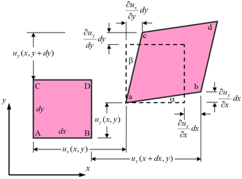 Two-dimensional geometric deformation of an infinitesimal material element.
As with stresses, strains may also be classified as 'normal strain' and 'shear strain' (i.e. acting perpendicular to or along the face of an element respectively). For an isotropic material that obeys Hooke's law, a normal stress will cause a normal strain. Normal strains produce dilations.
Consider a two-dimensional infinitesimal rectangular material element with dimensions
 , which after deformation, takes the form of a rhombus. From the geometry of the adjacent figure we have
and
For very small displacement gradients the squares of the derivatives are negligible and we have
The normal strain in the
 -direction of the rectangular element is defined by
Similarly, the normal strain in the
 -direction, and
  -direction, becomes
Shear strain
Shear strain SI symbol: γ or ϵ SI unit: 1, or radian Derivations from other quantities: γ = τ / G The engineering shear strain is defined as (γxy) is the change in angle between lines
 and
and  . Therefore,
From the geometry of the figure, we have
For small displacement gradients we have
For small rotations, i.e.
 and
and  are
are  we have
  . Therefore,
thus
By interchanging
and and  and
and  , it can be shown that
Similarly, for the
- and - planes, we haveThe tensorial shear strain components of the infinitesimal strain tensor can then be expressed using the engineering strain definition,
 , as
, asMetric tensor
A strain field associated with a displacement is defined, at any point, by the change in length of the tangent vectors representing the speeds of arbitrarily parametrized curves passing through that point.
A basic geometric result, due to Fréchet, von Neumann and Jordan, states that, if the lengths of the tangent vectors fulfill the axioms of a norm and the parallelogram law, then the length of a vector is the square root of the value of the quadratic form associated, by the polarization formula, with a positive definite bilinear map called the metric tensor.
Description of deformation
Deformation is the change in the metric properties of a continuous body, meaning that a curve drawn in the initial body placement changes its length when displaced to a curve in the final placement. If all the curves do not change length, it is said that a rigid body displacement occurred.
It is convenient to identify a reference configuration or initial geometric state of the continuum body which all subsequent configurations are referenced from. The reference configuration need not to be one the body actually will ever occupy. Often, the configuration at t = 0 is considered the reference configuration, κ0(B). The configuration at the current time t is the current configuration.
For deformation analysis, the reference configuration is identified as undeformed configuration, and the current configuration as deformed configuration. Additionally, time is not considered when analyzing deformation, thus the sequence of configurations between the undeformed and deformed configurations are of no interest.
The components Xi of the position vector X of a particle in the reference configuration, taken with respect to the reference coordinate system, are called the material or reference coordinates. On the other hand, the components xi of the position vector x of a particle in the deformed configuration, taken with respect to the spatial coordinate system of reference, are called the spatial coordinates
There are two methods for analysing the deformation of a continuum. One description is made in terms of the material or referential coordinates, called material description or Lagrangian description. A second description is of deformation is made in terms of the spatial coordinates it is called the spatial description or Eulerian description.
There is continuity during deformation of a continuum body in the sense that:
- The material points forming a closed curve at any instant will always form a closed curve at any subsequent time.
- The material points forming a closed surface at any instant will always form a closed surface at any subsequent time and the matter within the closed surface will always remain within.
Affine deformation
A deformation is called an affine deformation, if it can be described by an affine transformation. Such a transformation is composed of a linear transformation (such as rotation, shear, extension and compression) and a rigid body translation. Affine deformations are also called homogeneous deformations.[7]
Therefore an affine deformation has the form
where
 is the position of a point in the deformed configuration, is the position in a reference configuration, t is a time-like parameter,
  is the linear transformer and
  is the translation. In matrix form, where the components are with respect to an orthonormal basis,
The above deformation becomes non-affine or inhomogeneous if
 or
or  .
.Rigid body motion
A rigid body motion is a special affine deformation that does not involve any shear, extension or compression. The transformation matrix
is proper orthogonal in order to allow rotations but no reflections.A rigid body motion can be described by
where
In matrix form,
Displacement
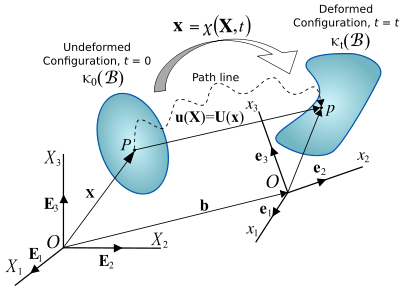 Figure 1. Motion of a continuum body.
A change in the configuration of a continuum body results in a displacement. The displacement of a body has two components: a rigid-body displacement and a deformation. A rigid-body displacement consist of a simultaneous translation and rotation of the body without changing its shape or size. Deformation implies the change in shape and/or size of the body from an initial or undeformed configuration
 to a current or deformed configuration
  (Figure 1).
If after a displacement of the continuum there is a relative displacement between particles, a deformation has occurred. On the other hand, if after displacement of the continuum the relative displacement between particles in the current configuration is zero, then there is no deformation and a rigid-body displacement is said to have occurred.
The vector joining the positions of a particle P in the undeformed configuration and deformed configuration is called the displacement vector u(X,t) = uiei in the Lagrangian description, or U(x,t) = UJEJ in the Eulerian description.
A displacement field is a vector field of all displacement vectors for all particles in the body, which relates the deformed configuration with the undeformed configuration. It is convenient to do the analysis of deformation or motion of a continuum body in terms of the displacement field, In general, the displacement field is expressed in terms of the material coordinates as
or in terms of the spatial coordinates as
where αJi are the direction cosines between the material and spatial coordinate systems with unit vectors EJ and ei, respectively. Thus
and the relationship between ui and UJ is then given by
Knowing that
then
It is common to superimpose the coordinate systems for the undeformed and deformed configurations, which results in b = 0, and the direction cosines become Kronecker deltas:
Thus, we have
or in terms of the spatial coordinates as
Displacement gradient tensor
The partial differentiation of the displacement vector with respect to the material coordinates yields the material displacement gradient tensor
 . Thus we have:
where
 is the deformation gradient tensor.
Similarly, the partial differentiation of the displacement vector with respect to the spatial coordinates yields the spatial displacement gradient tensor
 . Thus we have,
Examples of deformations
Homogeneous (or affine) deformations are useful in elucidating the behavior of materials. Some homogeneous deformations of interest are
- uniform extension
- pure dilation
- simple shear
- pure shear
Plane deformations are also of interest, particularly in the experimental context.
Plane deformation
A plane deformation, also called plane strain, is one where the deformation is restricted to one of the planes in the reference configuration. If the deformation is restricted to the plane described by the basis vectors
 , the deformation gradient has the form
In matrix form,
From the polar decomposition theorem, the deformation gradient, up to a change of coordinates, can be decomposed into a stretch and a rotation. Since all the deformation is in a plane, we can write[7]
where θ is the angle of rotation and λ1,λ2 are the principal stretches.
Isochoric plane deformation
If the deformation is isochoric (volume preserving) then
 and we have
- F11F22 − F12F21 = 1
Alternatively,
- λ1λ2 = 1
Simple shear
A simple shear deformation is defined as an isochoric plane deformation in which there are a set of line elements with a given reference orientation that do not change length and orientation during the deformation.[7]
If
 is the fixed reference orientation in which line elements do not deform during the deformation then λ1 = 1 and
  . Therefore,
Since the deformation is isochoric,
Define
 . Then, the deformation gradient in simple shear can be expressed as
Now,
Since
 we can also write the deformation gradient as
See also
- Deformation (engineering)
- Finite strain theory
- Infinitesimal strain theory
- Moiré pattern
- Shear modulus
- Shear stress
- Shear strength
- Stress (mechanics)
- Stress measures
References
- ^ a b Truesdell, C. and Noll, W., (2004), The non-linear field theories of mechanics: Third edition, Springer, p. 48.
- ^ H.-C. Wu, Continuum Mechanics and Plasticity, CRC Press (2005), ISBN 1-58488-363-4
- ^ Lubliner, Jacob (2008). Plasticity Theory (Revised Edition). Dover Publications. ISBN 0486462900. http://www.ce.berkeley.edu/~coby/plas/pdf/book.pdf.
- ^ a b Rees, David (2006). Basic Engineering Plasticity - An Introduction with Engineering and Manufacturing Applications. Butterworth-Heinemann. ISBN 0750680253. http://books.google.ca/books?id=4KWbmn_1hcYC.
- ^ "Earth."Encyclopædia Britannica from Encyclopædia Britannica 2006 Ultimate Reference Suite DVD .[2009].
- ^ Rees, David (2006). Basic Engineering Plasticity - An Introduction with Engineering and Manufacturing Applications. Butterworth-Heinemann. p. 41. ISBN 0750680253. http://books.google.ca/books?id=4KWbmn_1hcYC.
- ^ a b c Ogden, R. W., 1984, Non-linear Elastic Deformations, Dover.
Further reading
- Dill, Ellis Harold (2006). Continuum Mechanics: Elasticity, Plasticity, Viscoelasticity. Germany: CRC Press. ISBN 0849397790. http://books.google.com/?id=Nn4kztfbR3AC.
- Hutter, Kolumban; Klaus Jöhnk (2004). Continuum Methods of Physical Modeling. Germany: Springer. ISBN 3540206191. http://books.google.ca/books?id=B-dxx724YD4C.
- Lubarda, Vlado A. (2001). Elastoplasticity Theory. CRC Press. ISBN 0849311381. http://books.google.ca/books?id=1P0LybL4oAgC.
- Macosko, C. W. (1994). Rheology: principles, measurement and applications. VCH Publishers. ISBN 1-56081-579-5.
- Mase, George E. (1970). Continuum Mechanics. McGraw-Hill Professional. ISBN 0070406634. http://books.google.com/?id=bAdg6yxC0xUC.
- Mase, G. Thomas; George E. Mase (1999). Continuum Mechanics for Engineers (Second ed.). CRC Press. ISBN 0-8493-1855-6. http://books.google.com/?id=uI1ll0A8B_UC.
- Nemat-Nasser, Sia (2006). Plasticity: A Treatise on Finite Deformation of Heterogeneous Inelastic Materials. Cambridge: Cambridge University Press. ISBN 0521839793. http://books.google.ca/books?id=5nO78Rt0BtMC.
Categories:- Tensors
- Continuum mechanics
- Non-Newtonian fluids
- Solid mechanics
- Deformation


![\underline{\underline{\boldsymbol{\varepsilon}}} = \left[\begin{matrix}
\varepsilon_{xx} & \varepsilon_{xy} & \varepsilon_{xz} \\
\varepsilon_{yx} & \varepsilon_{yy} & \varepsilon_{yz} \\
\varepsilon_{zx} & \varepsilon_{zy} & \varepsilon_{zz} \\
\end{matrix}\right] = \left[\begin{matrix}
\varepsilon_{xx} & \gamma_{xy}/2 & \gamma_{xz}/2 \\
\gamma_{yx}/2 & \varepsilon_{yy} & \gamma_{yz}/2 \\
\gamma_{zx}/2 & \gamma_{zy}/2 & \varepsilon_{zz} \\
\end{matrix}\right]\,\!](6/4665e653f6f7b8070254f6614e527f86.png)


Wikimedia Foundation. 2010.