Orr–Sommerfeld equation

The Orr–Sommerfeld equation, in fluid dynamics, is an eigenvalue equation describing the linear two-dimensional modes of disturbance to a viscous parallel flow. The solution to the Navier–Stokes equations for a parallel, laminar flow can become unstable if certain conditions on the flow are satisfied, and the Orr–Sommerfeld equation determines precisely what the conditions for hydrodynamic stability are.

The equation is named after William McFadden Orr and Arnold Sommerfeld, who derived it at the beginning of the 20th century.

Formulation

A schematic diagram of the base state of the system. The flow under investigation represents a small perturbation away from this state. While the base state is parallel, the perturbation velocity has components in both directions.

The equation is derived by solving a linearized version of the Navier–Stokes equation for the perturbation velocity field

$\mathbf{u} = \left(U(z)+u'(x,z,t), 0 ,w'(x,z,t)\right)$,

where (U(z),0,0) is the unperturbed or basic flow. The perturbation velocity has the wave-like solution $\mathbf{u}' \propto \exp(i \alpha (x - c t))$ (real part understood). Using this knowledge, and the streamfunction representation for the flow, the following dimensional form of the Orr–Sommerfeld equation is obtained:

$\frac{\mu}{i\alpha\rho} \left({d^2 \over d z^2} - \alpha^2\right)^2 \varphi = (U - c)\left({d^2 \over d z^2} - \alpha^2\right) \varphi - U'' \varphi$,

where μ is the dynamic viscosity of the fluid, ρ is its density, and φ is the potential function. The equation can be written in non-dimensional form by measuring velocities according to a scale set by some characteristic velocity U₀, and by measuring lengths according to channel depth h. Then the equation takes the form

${1 \over i \alpha \, Re} \left({d^2 \over d z^2} - \alpha^2\right)^2 \varphi = (U - c)\left({d^2 \over d z^2} - \alpha^2\right) \varphi - U'' \varphi$,

where

$Re=\frac{\rho U_0 h}{\mu}$

is the Reynolds number of the base flow. The relevant boundary conditions are the no-slip boundary conditions at the channel top and bottom z = z₁ and z = z₂,

$\alpha \varphi = {d \varphi \over d z} = 0$ at z = z₁ and z = z₂.

The eigenvalue parameter of the problem is c and the eigenvector is φ. If the imaginary part of the wave speed c is positive, then the base flow is unstable, and the small perturbation introduced to the system is amplified in time.

Solutions

For all but the simplest of velocity profiles U, numerical or asymptotic methods are required to calculate solutions. Some typical flow profiles are discussed below. In general, the spectrum of the equation is discrete and infinite for a bounded flow, while for unbounded flows (such as boundary-layer flow), the spectrum contains both continuous and discrete parts^[1].

The spectrum of the Orr–Sommerfeld for Poiseuille flow at criticality.

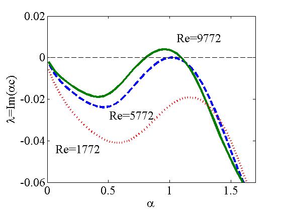
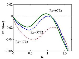Dispersion curves of the Poiseuille flow for various Reynolds numbers.

For plane Poiseuille flow, it has been shown that the flow is unstable (i.e. one or more eigenvalues c has a positive imaginary part) for some α when Re > Re_c = 5772.22 and the neutrally stable mode at Re = Re_c having α_c = 1.02056, c_r = 0.264002.^[2] To see the stability properties of the system, it is customary to plot a dispersion curve, that is, a plot of the growth rate Im(αc) as a function of the wavenumber α.

The first figure shows the spectrum of the Orr–Sommerfeld equation at the critical values listed above. This is a plot of the eigenvalues (in the form λ = − iαc) in the complex plane. The rightmost eigenvalue is the most unstable one. At the critical values of Reynolds number and wavenumber, the rightmost eigenvalue is exactly zero. For higher (lower) values of Reynolds number, the rightmost eigenvalue shifts into the positive (negative) half of the complex plane. Then, a fuller picture of the stability properties is given by a plot exhibiting the functional dependence of this eigenvalue; this is shown in the second figure.

On the other hand, the spectrum of eigenvalues for Couette flow indicates stability, at all Reynolds numbers^[3]. However, in experiments, Couette flow is found to be unstable to small, but finite, perturbations for which the linear theory, and the Orr-Sommerfeld equation do not apply. It has been argued that the non-normality of the eigenvalue problem associated with Couette (and indeed, Poiseuille) flow^[4] might explain that observed instability. That is, the eigenfunctions of the Orr–Sommerfeld operator are complete but non-orthogonal. Then, the energy of the disturbance contains contributions from all eigenfunctions of the Orr–Sommerfeld equation. Even if the energy associated with each eigenvalue considered separately is decaying exponentially in time (as predicted by the Orr–Sommerfeld analysis for the Couette flow), the cross terms arising from the non-orthogonality of the eigenvalues can increase transiently. Thus, the total energy increases transiently (before tending asymptotically to zero). The argument is that if the magnitude of this transient growth is sufficiently large, it destabilizes the laminar flow, however this argument has been criticized ^[5] since it invoques finite amplitudes in the context of a linear (that is zero amplitude) theory. A true explanation of instability in Couette and other shear flows such as Pipe and channel flows must include nonlinear effects.

A nonlinear theory ^[6], ^[7] has been proposed instead. Although that theory does include linear transient growth, the focus is on elucidating the key 3D nonlinear process underlying transition and turbulence in shear flows. That nonlinear theory has led to the construction of complete 3D steady states, traveling waves and time-periodic solutions of the Navier-Stokes equations that capture many of the key features of transition and coherent structures observed in the near wall region of turbulent shear flows. ^{[8] [9] [10] [11] [12] [13]}

Mathematical methods for free-surface flows

For Couette flow, it is possible to make mathematical progress in the solution of the Orr–Sommerfeld equation. In this section, a demonstration of this method is given for the case of free-surface flow, that is, when the upper lid of the channel is replaced by a free surface. Note first of all that it is necessary to modify upper boundary conditions to take account of the free surface. In non-dimensional form, these conditions now read

$\varphi={d \varphi \over d z}=0,$ at z = 0,

$\frac{d^2\varphi}{dz^2}+\alpha^2\varphi=0$, $\Omega\equiv\frac{d^3\varphi}{dz^3}+i\alpha Re\left[\left(c-U\left(z_2=1\right)\right)\frac{d\varphi}{dz}+\varphi\right]-i\alpha Re\left(\frac{1}{Fr}+\frac{\alpha^2}{We}\right)\frac{\varphi}{c-U\left(z_2=1\right)}=0,$ at $\,z=1$.

The first free-surface condition is the statement of continuity of tangential stress, while the second condition relates the normal stress to the surface tension. Here

$Fr=\frac{U_0^2}{gh},\,\,\ We=\frac{\rho u_0^2 h}{\sigma}$

are the Froude and Weber numbers respectively.

For Couette flow $U\left(z\right)=z$, the four linearly independent solutions to the non-dimensional Orr–Sommerfeld equation are^[14],

$\chi_1\left(z\right)=\sinh\left(\alpha z\right),\qquad \chi_2\left(z\right)=\cosh\left(\alpha z\right)$,

$\chi_3\left(z\right)=\frac{1}{\alpha}\int_\infty^z\sinh\left[\alpha\left(z-\xi\right)\right]Ai\left[e^{i\pi/6}\left(\alpha Re\right)^{1/3}\left(\xi-c-\frac{i\alpha}{Re}\right)\right]d\xi,$

$\chi_4\left(z\right)=\frac{1}{\alpha}\int_\infty^z\sinh\left[\alpha\left(z-\xi\right)\right]Ai\left[e^{5i\pi/6}\left(\alpha Re\right)^{1/3}\left(\xi-c-\frac{i\alpha}{Re}\right)\right]d\xi,$

where $Ai\left(\cdot\right)$ is the Airy function of the first kind. Substitution of the superposition solution $\varphi=\sum_{i=1}^4 c_i\chi_i\left(z\right)$ into the four boundary conditions gives four equations in the four unknown constants c_i. For the equations to have a non-trivial solution, the determinant condition

$\left|\begin{array}{cccc}\chi_1\left(0\right)&\chi_2\left(0\right)&\chi_3\left(0\right)&\chi_4\left(0\right)\\ \chi_1'\left(0\right)&\chi_2'\left(0\right)&\chi_3'\left(0\right)&\chi_4'\left(0\right)\\ \Omega_1\left(1\right)&\Omega_2\left(1\right)&\Omega_3\left(1\right)&\Omega_4\left(1\right)\\ \chi_1''\left(1\right)+\alpha^2\chi_1\left(1\right)&\chi_2''\left(1\right)+\alpha^2\chi_2\left(1\right)&\chi_3''\left(1\right)+\alpha^2\chi_3\left(1\right)&\chi_4''\left(1\right)+\alpha^2\chi_4\left(1\right)\end{array}\right|=0$

must be satisfied. This is a single equation in the unknown c, which can be solved numerically or by asymptotic methods. It can be shown that for a range of wavenumbers α and for sufficiently large Reynolds numbers, the growth rate αc_i is positive. Edit: the notation αc for the growth rate is not clear.

References

Historical

• Orr, W. M'F. (1907), "The stability or instability of the steady motions of a liquid. Part I", Proceedings of the Royal Irish Academy, A 27: 9–68 
• Orr, W. M'F. (1907), "The stability or instability of the steady motions of a liquid. Part II", Proceedings of the Royal Irish Academy, A 27: 69–138 
• Sommerfeld, A. (1908), "Ein Beitrag zur hydrodynamische Erklärung der turbulenten Flüssigkeitsbewegungen", Proceedings of the 4th International Congress of Mathematicians, III, Rome, pp. 116–124 

Further reading

1. ^ A. P. Hooper and R. Grimshaw (1996) 'Two-dimensional disturbance growth of linearly stable viscous shear flows' Phys. Fluids 8, 1424
2. ^ Orszag S. A. (1971) 'Accurate solution of the Orr–Sommerfeld stability equation' J. Fluid. Mech. 50, 689–703
3. ^ P. G. Drazin and W. H. Reid (1981) 'Hydrodynamic Stability' Cambridge University Press
4. ^ N. L. Trefethen, A. E. Trefethen, S. C. Teddy and T. A. Driscoll (1993) 'Hydrodynamic stability without eigenvalues' Science, 261, 578–584
5. ^ Fabian Waleffe (1995) `Transition in shear flows: Nonlinear normality versus non-normal linearity.' Physics of Fluids 7, pp. 3060-3066.
6. ^ Fabian Waleffe (1995) `Hydrodynamic Stability and Turbulence: Beyond transients to a self-sustaining process' Studies in Applied Mathematics, 95, pp. 319-343
7. ^ Fabian Waleffe (1997) `On a self-sustaining process in shear flows', Physics of Fluids, Vol. 9, pp. 883-900
8. ^ Fabian Waleffe (1998) `Three-Dimensional Coherent States in Plane Shear Flows' Physical Review Letters, Vol. 81, Number 19, pp. 4140-4143
9. ^ Fabian Waleffe (2001) `Exact Coherent Structures in Channel Flow' Journal of Fluid Mechnaics, Vol. 435, pp. 93-102 (May 2001)
10. ^ Fabian Waleffe (2003) `Homotopy of exact coherent structures in plane shear flows' Physics of Fluids, 15, pp. 1517-1534
11. ^ Holger Faisst and Bruno Eckhardt (2003) `Traveling Waves in Pipe Flow' Phys. Rev. Lett. 91, 224502
12. ^ Wedin and Kerswell (2004) `Exact coherent states in pipe flow', Journal of Fluid Mechanics, 508:333-371
13. ^ B. Hof,C. W. H. van Doorne1, J. Westerweel, F.T.M. Nieuwstadt1, H. Faisst, B. Eckhardt, H. Wedin, R.R. Kerswell and F. Waleffe, `Experimental Observation of Nonlinear Traveling Waves in Turbulent Pipe Flow' Science, 10 September 2004: Vol. 305 no. 5690, pp. 1594-1598
14. ^ R. Miesen and B. J. Boersma (1995) 'Hydrodynamic stability of a sheared liquid film' Journal of Fluid Mechanics, 301, 175–202