Daubechies wavelet

Daubechies 20 2-d wavelet (Wavelet Fn X Scaling Fn)

Named after Ingrid Daubechies, the Daubechies wavelets are a family of orthogonal wavelets defining a discrete wavelet transform and characterized by a maximal number of vanishing moments for some given support. With each wavelet type of this class, there is a scaling function (also called father wavelet) which generates an orthogonal multiresolution analysis.

Properties

In general the Daubechies wavelets are chosen to have the highest number A of vanishing moments, (this does not imply the best smoothness) for given support width N=2A, and among the 2^A−1 possible solutions the one is chosen whose scaling filter has extremal phase. The wavelet transform is also easy to put into practice using the fast wavelet transform. Daubechies wavelets are widely used in solving a broad range of problems, e.g. self-similarity properties of a signal or fractal problems, signal discontinuities, etc.

The Daubechies wavelets are not defined in terms of the resulting scaling and wavelet functions; in fact, they are not possible to write down in closed form. The graphs below are generated using the cascade algorithm, a numeric technique consisting of simply inverse-transforming [1 0 0 0 0 ... ] an appropriate number of times.

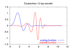
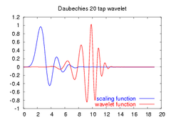
scaling and wavelet functions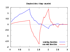
amplitudes of the frequency spectra of the above functions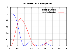

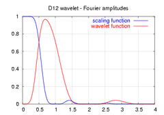
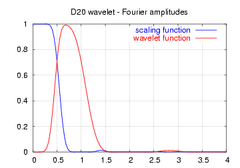
Note that the spectra shown here are not the frequency response of the high and low pass filters, but rather the amplitudes of the continuous Fourier transforms of the scaling (blue) and wavelet (red) functions.

Daubechies orthogonal wavelets D2-D20 (even index numbers only) are commonly used. The index number refers to the number N of coefficients. Each wavelet has a number of zero moments or vanishing moments equal to half the number of coefficients. For example, D2 (the Haar wavelet) has one vanishing moment, D4 has two, etc. A vanishing moment limits the wavelet's ability to represent polynomial behaviour or information in a signal. For example, D2, with one moment, easily encodes polynomials of one coefficient, or constant signal components. D4 encodes polynomials with two coefficients, i.e. constant and linear signal components; and D6 encodes 3-polynomials, i.e. constant, linear and quadratic signal components. This ability to encode signals is nonetheless subject to the phenomenon of scale leakage, and the lack of shift-invariance, which arise from the discrete shifting operation (below) during application of the transform. Sub-sequences which represent linear, quadratic (for example) signal components are treated differently by the transform depending on whether the points align with even- or odd-numbered locations in the sequence. The lack of the important property of shift-invariance, has led to the development of several different versions of a shift-invariant (discrete) wavelet transform.

Construction

Both the scaling sequence (Low-Pass Filter) and the wavelet sequence (Band-Pass Filter) (see orthogonal wavelet for details of this construction) will here be normalized to have sum equal 2 and sum of squares equal 2. In some applications, they are normalised to have sum $\sqrt{2}$, so that both sequences and all shifts of them by an even number of coefficients are orthonormal to each other.

Using the general representation for a scaling sequence of an orthogonal discrete wavelet transform with approximation order A,

$a(Z)=2^{1-A}(1+Z)^A\,p(Z)$, with N=2A, p having real coefficients, p(1)=1 and degree(p)=A-1,

one can write the orthogonality condition as

$a(Z)\,a(Z^{-1})+a(-Z)\,a(-Z^{-1})=4$, or equally as $(2-X)^A P(X)+X^A\,P(2-X)=2^A$ (*),

with the Laurent-polynomial $X:=1/2\cdot(2-Z-Z^{-1})$ generating all symmetric sequences and X( − Z) = 2 − X(Z). Further, P(X) stands for the symmetric Laurent-polynomial P(X(Z)) = p(Z)p(Z ^{− 1}). Since X(e^iw) = 1 − cos(w) and p(e^iw)p(e ^{− iw}) = | p(e^iw) | ², P takes nonnegative values on the segment [0,2].

Equation (*) has one minimal solution for each A, which can be obtained by division in the ring of truncated power series in X,

$P_A(X)=\sum_{k=0}^{A-1}\left({{A+k-1}\atop{A-1}}\right)2^{-k}X^k$.

Obviously, this has positive values on (0,2)

The homogeneous equation for (*) is antisymmetric about X=1 and has thus the general solution X^A(X − 1)R((X − 1)²), with R some polynomial with real coefficients. That the sum

P(X) = P_A(X) + X^A(X − 1)R((X − 1)²)

shall be nonnegative on the interval [0,2] translates into a set of linear restrictions on the coefficients of R. The values of P on the interval [0,2] are bounded by some quantity 4^{A − r}, maximizing r results in a linear program with infinitely many inequality conditions.

To solve P(X(Z)) = p(Z)p(Z ^{− 1}) for p one uses a technique called spectral factorization resp. Fejer-Riesz-algorithm. The polynomial P(X) splits into linear factors $P(X)=(X-\mu_1)\dots(X-\mu_N)$, N=A+1+2deg(R). Each linear factor represents a Laurent-polynomial $(X(Z)-\mu)=-\frac12Z+1-\mu-\frac12Z^{-1}$ that can be factored into two linear factors. One can assign either one of the two linear factors to p(Z), thus one obtains 2^N possible solutions. For extremal phase one chooses the one that has all complex roots of p(Z) inside or on the unit circle and is thus real.

The scaling sequences of lowest approximation order

Below are the coefficients for the scaling functions for D2-20. The wavelet coefficients are derived by reversing the order of the scaling function coefficients and then reversing the sign of every second one, (i.e., D4 wavelet = {-0.1830127, -0.3169873, 1.1830127, -0.6830127}). Mathematically, this looks like b_k = ( − 1)^ka_{N − 1 − k} where k is the coefficient index, b is a coefficient of the wavelet sequence and a a coefficient of the scaling sequence. N is the wavelet index, i.e., 2 for D2.

Orthogonal Daubechies coefficients (normalized to have sum 2)

D2 (Haar)	D4	D6	D8	D10	D12	D14	D16	D18	D20
1	0.6830127	0.47046721	0.32580343	0.22641898	0.15774243	0.11009943	0.07695562	0.05385035	0.03771716
1	1.1830127	1.14111692	1.01094572	0.85394354	0.69950381	0.56079128	0.44246725	0.34483430	0.26612218
	0.3169873	0.650365	0.8922014	1.02432694	1.06226376	1.03114849	0.95548615	0.85534906	0.74557507
	-0.1830127	-0.19093442	-0.03957503	0.19576696	0.44583132	0.66437248	0.82781653	0.92954571	0.97362811
		-0.12083221	-0.26450717	-0.34265671	-0.31998660	-0.20351382	-0.02238574	0.18836955	0.39763774
		0.0498175	0.0436163	-0.04560113	-0.18351806	-0.31683501	-0.40165863	-0.41475176	-0.35333620
			0.0465036	0.10970265	0.13788809	0.1008467	6.68194092e-4	-0.13695355	-0.27710988
			-0.01498699	-0.00882680	0.03892321	0.11400345	0.18207636	0.21006834	0.18012745
				-0.01779187	-0.04466375	-0.05378245	-0.02456390	0.043452675	0.13160299
				4.71742793e-3	7.83251152e-4	-0.02343994	-0.06235021	-0.09564726	-0.10096657
					6.75606236e-3	0.01774979	0.01977216	3.54892813e-4	-0.04165925
					-1.52353381e-3	6.07514995e-4	0.01236884	0.03162417	0.04696981
						-2.54790472e-3	-6.88771926e-3	-6.67962023e-3	5.10043697e-3
						5.00226853e-4	-5.54004549e-4	-6.05496058e-3	-0.01517900
							9.55229711e-4	2.61296728e-3	1.97332536e-3
							-1.66137261e-4	3.25814671e-4	2.81768659e-3
								-3.56329759e-4	-9.69947840e-4
								5.5645514e-5	-1.64709006e-4
									1.32354367e-4
									-1.875841e-5

Parts of the construction are also used to derive the biorthogonal Cohen-Daubechies-Feauveau wavelets (CDFs).

Implementation

While software such as Mathematica supports Daubechies wavelets directly^[1] a basic implementation is simple in MATLAB (in this case, Daubechies 4). This implementation uses periodization to handle the problem of finite length signals. Other, more sophisticated methods are available, but often it is not necessary to use these as it only affects the very ends of the transformed signal. The periodization is accomplished in the forward transform directly in MATLAB vector notation, and the inverse transform by using the circshift() function:

Transform, D4

It is assumed that S, a column vector with an even number of elements, has been pre-defined as the signal to be analyzed.

N = length(S);
s1 = S(1:2:N-1) + sqrt(3)*S(2:2:N);
d1 = S(2:2:N) - sqrt(3)/4*s1 - (sqrt(3)-2)/4*[s1(N/2); s1(1:N/2-1)];
s2 = s1 - [d1(2:N/2); d1(1)];
s = (sqrt(3)-1)/sqrt(2) * s2;
d = (sqrt(3)+1)/sqrt(2) * d1;

Inverse transform, D4

d1 = d * ((sqrt(3)-1)/sqrt(2));
s2 = s * ((sqrt(3)+1)/sqrt(2));
s1 = s2 + circshift(d1,-1);
S(2:2:N) = d1 + sqrt(3)/4*s1 + (sqrt(3)-2)/4*circshift(s1,1);
S(1:2:N-1) = s1 - sqrt(3)*S(2:2:N);

See also

• Binomial-QMF (Daubechies Wavelet Filters)
• Fast wavelet transform

References

1. ^ Daubechies Wavelet in Mathematica

• Jensen; la Cour-Harbo (2001). Ripples in Mathematics. Berlin: Springer. pp. 157–160. ISBN 3-540-41662-5. http://www.control.auc.dk/~alc/ripples.html. 

• Jianhong Shen and Gilbert Strang, Applied and Computational Harmonic Analysis, 5(3), Asymptotics of Daubechies Filters, Scaling Functions, and Wavelets.

External links

• Ingrid Daubechies: Ten Lectures on Wavelets, SIAM 1992
• A.N. Akansu, An Efficient QMF-Wavelet Structure (Binomial-QMF Daubechies Wavelets), Proc. 1st NJIT Symposium on Wavelets, April 1990
• Proc. 1st NJIT Symposium on Wavelets, Subbands and Transforms, April 1990
• Carlos Cabrelli, Ursula Molter: Generalized Self-similarity", Journal of Mathematical Analysis and Applications, 230: 251 - 260, 1999.
• Hardware implementation of wavelets
• I. Kaplan, The Daubechies D4 Wavelet Transform.