Renormalization group

In theoretical physics, the renormalization group (RG) refers to a mathematical apparatus that allows systematic investigation of the changes of a physical system as viewed at different distance scales. In particle physics, it reflects the changes in the underlying force laws (codified in a quantum field theory) as the energy scale at which physical processes occur varies, energy/momentum and resolution distance scales being effectively conjugate under the uncertainty principle (cf. Compton wavelength).

A change in scale is called a "scale transformation". The renormalization group is intimately related to "scale invariance" and "conformal invariance", symmetries in which a system appears the same at all scales (so-called self-similarity). (However, note that scale transformations are included in conformal transformations, in general: the latter including additional symmetry generators associated with special conformal transformations.)

As the scale varies, it is as if one is changing the magnifying power of a notional microscope viewing the system. In so-called renormalizable theories, the system at one scale will generally be seen to consist of self-similar copies of itself when viewed at a smaller scale, with different parameters describing the components of the system. The components, or fundamental variables, may relate to atoms, elementary particles, atomic spins, etc. The parameters of the theory typically describe the interactions of the components. These may be variable "couplings" which measure the strength of various forces, or mass parameters themselves. The components themselves may appear to be composed of more of the self-same components as one goes to shorter distances.

For example, in quantum electrodynamics (QED), an electron appears to be composed of electrons, positrons (anti-electrons) and photons, as one views it at higher resolution, at very short distances. The electron at such short distances has a slightly different electric charge than does the "dressed electron" seen at large distances, and this change, or "running," in the value of the electric charge is determined by the renormalization group equation.

History of the renormalization group

The idea of scale transformations and scale invariance is old in physics. Scaling arguments were commonplace for the Pythagorean school, Euclid and up to Galileo.^{[citation needed]} They became popular again at the end of the 19th century, perhaps the first example being the idea of enhanced viscosity of Osborne Reynolds, as a way to explain turbulence.

The renormalization group was initially devised in particle physics, but nowadays its applications extend to solid-state physics, fluid mechanics, cosmology and even nanotechnology. An early article by Ernst Stueckelberg and Andre Petermann in 1953 anticipates the idea in quantum field theory. Stueckelberg and Petermann opened the field conceptually. They noted that renormalization exhibits a group of transformations which transfer quantities from the bare terms to the counterterms. They introduced a function h(e) in QED, which is now called the beta function (see below).

Murray Gell-Mann and Francis E. Low in 1954 restricted the idea to scale transformations in QED, which are the most physically significant, and focused on asymptotic forms of the photon propagator at high energies. They determined the variation of the electromagnetic coupling in QED, by appreciating the simplicity of the scaling structure of that theory. They thus discovered that the coupling parameter g(μ) at the energy scale μ is effectively given by the group equation

g(μ) = G⁻¹( (μ/M)^d G(g(M)) ) ,

for some function G and a constant d, in terms of the coupling at a reference scale M. Gell-Mann and Low realized in these results that the effective scale can be arbitrarily taken as μ, and can vary to define the theory at any other scale:

g(κ) = G⁻¹( (κ/μ)^d G(g(μ)) ) = G⁻¹( (κ/M)^d G(g(M)) ) .

The gist of the RG is this group property: as the scale μ varies, the theory presents a self-similar replica of itself, and any scale can be accessed similarly from any other scale, by group action, a formal conjugacy of couplings in the mathematical sense (Schröder's equation).

On the basis of this (finite) group equation, Gell-Mann and Low then focussed on infinitesimal transformations, and invented a computational method based on a mathematical flow function ψ(g) = G d/(∂G/∂g) of the coupling parameter g, which they introduced. Like the function h(e) of Stueckelberg and Petermann, their function determines the differential change of the coupling g(μ) with respect to a small change in energy scale μ through a differential equation, the renormalization group equation:

∂g / ∂ln(μ) = ψ(g) = β(g) .

The modern name is also indicated, the beta function, introduced by C. Callan and K. Symanzik in the early 1970s. Since it is a mere function of g, integration in g of a perturbative estimate of it permits specification of the renormalization trajectory of the coupling, that is, its variation with energy, effectively the function G in this perturbative approximation. The renormalization group prediction (cf Stueckelberg-Petermann and Gell-Mann-Low works) was confirmed 40 years later at the LEP accelerator experiments: the fine structure "constant" of QED was measured to be about 1/127 at energies close to 200 GeV, as opposed to the standard low-energy physics value of 1/137. (Early applications to quantum electrodynamics are discussed in the influential book of Nikolay Bogolyubov and Dmitry Shirkov in 1959.)

The renormalization group emerges from the renormalization of the quantum field variables, which normally has to address the problem of infinities in a quantum field theory (although the RG exists independently of the infinities). This problem of systematically handling the infinities of quantum field theory to obtain finite physical quantities was solved for QED by Richard Feynman, Julian Schwinger and Sin-Itiro Tomonaga, who received the 1965 Nobel prize for these contributions. They effectively devised the theory of mass and charge renormalization, in which the infinity in the momentum scale is cut-off by an ultra-large regulator, Λ (which could ultimately be taken to be infinite — infinities reflect the pileup of contributions from an infinity of degrees of freedom at infinitely high energy scales.). The dependence of physical quantities, such as the electric charge or electron mass, on the scale Λ is hidden, effectively swapped for the longer-distance scales at which the physical quantities are measured, and, as a result, all observable quantities end up being finite, instead, even for an infinite Λ. Gell-Mann and Low thus realized in these results that, while, infinitesimally, a tiny change in g is provided by the above RG equation given ψ(g), the self-similarity is expressed by the fact that ψ(g) depends explicitly only upon the parameter(s) of the theory, and not upon the scale μ. Consequently, the above renormalization group equation may be solved for (G and thus) g(μ).

A deeper understanding of the physical meaning and generalization of the renormalization process, which goes beyond the dilatation group of conventional renormalizable theories, came from condensed matter physics. Leo P. Kadanoff's paper in 1966 proposed the "block-spin" renormalization group. The blocking idea is a way to define the components of the theory at large distances as aggregates of components at shorter distances.

This approach covered the conceptual point and was given full computational substance in the extensive important contributions of Kenneth Wilson. The power of Wilson's ideas was demonstrated by a constructive iterative renormalization solution of a long-standing problem, the Kondo problem, in 1974, as well as the preceding seminal developments of his new method in the theory of second-order phase transitions and critical phenomena in 1971. He was awarded the Nobel prize for these decisive contributions in 1982. (The connection between the Stueckelberg-Petermann and the Wilson renormalization groups has also been discussed by M. Duetsch, arXiv:1012.5604.)

Meanwhile, the RG in particle physics had been reformulated in more practical terms by C. G. Callan and K. Symanzik in 1970. The above beta function, which describes the "running of the coupling" parameter with scale, was also found to amount to the "canonical trace anomaly", which represents the quantum-mechanical breaking of scale (dilation) symmetry in a field theory. (Remarkably, quantum mechanics itself can induce mass through the trace anomaly and the running coupling.) Applications of the RG to particle physics exploded in number in the 1970s with the establishment of the Standard Model.

In 1973, it was discovered that a theory of interacting colored quarks, called quantum chromodynamics had a negative beta function. This means that an initial high-energy value of the coupling will eventuate a special value of μ at which the coupling blows up (diverges). This special value is the scale of the strong interactions, μ = Λ_QCD and occurs at about 200 MeV. Conversely, the coupling becomes weak at very high energies (asymptotic freedom), and the quarks become observable as point-like particles, in deep inelastic scattering, as anticipated by Feynman-Bjorken scaling. QCD was thereby established as the quantum field theory controlling the strong interactions of particles.

Momentum space RG also became a highly developed tool in solid state physics, but its success was hindered by the extensive use of perturbation theory, which prevented the theory from reaching success in strongly correlated systems. In order to study these strongly correlated systems, variational approaches are a better alternative. During the 1980s some real-space RG techniques were developed in this sense, the most successful being the density-matrix RG (DMRG), developed by S. R. White and R. M. Noack in 1992.

The conformal symmetry is associated with the vanishing of the beta function. This can occur naturally if a coupling constant is attracted, by running, toward a fixed point at which β(g) = 0. In QCD, the fixed point occurs at short distances where g → 0 and is called a (trivial) ultraviolet fixed point. For heavy quarks, such as the top quark, it is calculated that the coupling to the mass-giving Higgs boson runs toward a fixed non-zero (non-trivial) infrared fixed point.

In string theory conformal invariance of the string world-sheet is a fundamental symmetry: β=0 is a requirement. Here, β is a function of the geometry of the space-time in which the string moves. This determines the space-time dimensionality of the string theory and enforces Einstein's equations of general relativity on the geometry. The RG is of fundamental importance to string theory and theories of grand unification.

It is also the modern key idea underlying critical phenomena in condensed matter physics. Indeed, the RG has become one of the most important tools of modern physics. It is often used^[1] in combination with the Monte Carlo method.

Block spin renormalization group

This section introduces pedagogically a picture of RG which may be easiest to grasp: the block spin RG. It was devised by Leo P. Kadanoff in 1966.

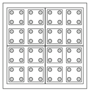
Let us consider a 2D solid, a set of atoms in a perfect square array, as depicted in the figure. Let us assume that atoms interact among themselves only with their nearest neighbours, and that the system is at a given temperature T. The strength of their interaction is measured by a certain coupling constant J. The physics of the system will be described by a certain formula, say H(T,J).

Now we proceed to divide the solid into blocks of $2\times 2$ squares; we attempt to describe the system in terms of block variables, i.e.: some variables which describe the average behavior of the block. Also, let us assume that, due to a lucky coincidence, the physics of block variables is described by a formula of the same kind, but with different values for T and J: H(T',J'). (This isn't exactly true, of course, but it is often approximately true in practice, and that is good enough, to a first approximation.)

Perhaps the initial problem was too hard to solve, since there were too many atoms. Now, in the renormalized problem we have only one fourth of them. But why should we stop now? Another iteration of the same kind leads to H(T'',J''), and only one sixteenth of the atoms. We are increasing the observation scale with each RG step.

Of course, the best idea is to iterate until there is only one very big block. Since the number of atoms in any real sample of material is very large, this is more or less equivalent to finding the long term behaviour of the RG transformation which took $(T,J)\to (T',J')$ and $(T',J')\to (T'',J'')$. Usually, when iterated many times, this RG transformation leads to a certain number of fixed points.

Let us be more concrete and consider a magnetic system (e.g.: the Ising model), in which the J coupling constant denotes the trend of neighbour spins to be parallel. The configuration of the system is the result of the tradeoff between the ordering J term and the disordering effect of temperature. For many models of this kind there are three fixed points:

1. T = 0 and $J\to\infty$. This means that, at the largest size, temperature becomes unimportant, i.e.: the disordering factor vanishes. Thus, in large scales, the system appears to be ordered. We are in a ferromagnetic phase.
2. $T\to\infty$ and $J\to 0$. Exactly the opposite, temperature dominates, and the system is disordered at large scales.
3. A nontrivial point between them, T = T_c and J = J_c. In this point, changing the scale does not change the physics, because the system is in a fractal state. It corresponds to the Curie phase transition, and is also called a critical point.

So, if we are given a certain material with given values of T and J, all we have to do in order to find out the large scale behaviour of the system is to iterate the pair until we find the corresponding fixed point.

Elements of RG theory

In more technical terms, let us assume that we have a theory described by a certain function Z of the state variables {s_i} and a certain set of coupling constants {J_k}. This function may be a partition function, an action, a Hamiltonian, etc. It must contain the whole description of the physics of the system.

Now we consider a certain blocking transformation of the state variables $\{s_i\}\to \{\tilde s_i\}$, the number of $\tilde s_i$ must be lower than the number of s_i. Now let us try to rewrite the Z function only in terms of the $\tilde s_i$. If this is achievable by a certain change in the parameters, $\{J_k\}\to \{\tilde J_k\}$, then the theory is said to be renormalizable.

For some reason, most fundamental theories of physics such as quantum electrodynamics, quantum chromodynamics and electro-weak interaction, but not gravity, are exactly renormalizable. Also, most theories in condensed matter physics are approximately renormalizable, from superconductivity to fluid turbulence.

The change in the parameters is implemented by a certain beta function: $\{\tilde J_k\}=\beta(\{ J_k \})$, which is said to induce a renormalization flow (or RG flow) on the J-space. The values of J under the flow are called running couplings.

As was stated in the previous section, the most important information in the RG flow are its fixed points. The possible macroscopic states of the system, at a large scale, are given by this set of fixed points.

Since the RG transformations in such systems are lossy (i.e.: the number of variables decreases - see as an example in a different context, Lossy data compression), there need not be an inverse for a given RG transformation. Thus, in such lossy systems, the renormalization group is, in fact, a semigroup.

Relevant and irrelevant operators, universality classes

Let us consider a certain observable A of a physical system undergoing an RG transformation. The magnitude of the observable as the length scale of the system goes from small to large may be (a) always increasing, (b) always decreasing or (c) other. In the first case, the observable is said to be a relevant observable; in the second, irrelevant and in the third, marginal.

A relevant operator is needed to describe the macroscopic behaviour of the system; an irrelevant observable is not. Marginal observables may or may not need to be taken into account. A remarkable fact is that most observables are irrelevant, i.e.: the macroscopic physics is dominated by only a few observables in most systems. In other terms: microscopic physics contains $\approx 10^{23}$ (Avogadro's number) variables, and macroscopic physics only a few.

Before the RG, there was an astonishing empirical fact to explain: the coincidence of the critical exponents (i.e.: the behaviour near a second order phase transition) in very different phenomena, such as magnetic systems, superfluid transition (Lambda transition), alloy physics, etc. This was called universality and is successfully explained by RG, just showing that the differences between all those phenomena are related to irrelevant observables.

Thus, many macroscopic phenomena may be grouped into a small set of universality classes, described by the set of relevant observables.

See also: Dangerously irrelevant operator

Momentum space RG

RG, in practice, comes in two main flavours. The Kadanoff picture explained above refers mainly to the so-called real-space RG. Momentum-space RG on the other hand, has a longer history despite its relative subtlety.^{[citation needed]} It can be used for systems where the degrees of freedom can be cast in terms of the Fourier modes of a given field. The RG transformation proceeds by integrating out a certain set of high momentum (large wavenumber) modes. Since large wavenumbers are related to short length scales, the momentum-space RG results in an essentially similar coarse-graining effect as with real-space RG.

Momentum-space RG is usually performed on a perturbation expansion. The validity of such an expansion is predicated upon the true physics of our system being close to that of a free field system. In this case, we may calculate observables by summing the leading terms in the expansion. This approach has proved very successful for many theories, including most of particle physics, but fails for systems whose physics is very far from any free system, i.e., systems with strong correlations.

As an example of the physical meaning of RG in particle physics we will give a short description of charge renormalization in quantum electrodynamics (QED). Let us suppose we have a point positive charge of a certain true (or bare) magnitude. The electromagnetic field around it has a certain energy, and thus may produce some pairs of (e.g.) electrons-positrons, which will be annihilated very quickly. But in their short life, the electron will be attracted by the charge, and the positron will be repelled. Since this happens continuously, these pairs are effectively screening the charge from abroad. Therefore, the measured strength of the charge will depend on how close to our probes it may enter. We have a dependence of a certain coupling constant (the electric charge) with distance.

Momentum and length scales are related inversely according to the de Broglie relation: the higher the energy or momentum scale we may reach, the lower the length scale we may probe and resolve. Therefore, the momentum-space RG practitioners sometimes declaim to integrate out high momenta or high energy from their theories.

Appendix: Exact Renormalization Group Equations

An exact renormalization group equation (ERGE) is one that takes irrelevant couplings into account. There are several formulations.

The Wilson ERGE is the simplest conceptually, but is practically impossible to implement. Fourier transform into momentum space after Wick rotating into Euclidean space. Insist upon a hard momentum cutoff, $p^2 \leq \Lambda^2$ so that the only degrees of freedom are those with momenta less than Λ. The partition function is

$Z=\int_{p^2\leq \Lambda^2} \mathcal{D}\phi \exp\left[-S_\Lambda(\phi)\right].$

For any positive Λ′ less than Λ, define S_Λ′ (a functional over field configurations φ whose Fourier transform has momentum support within $p^2 \leq \Lambda'^2$) as

$\exp\left(-S_{\Lambda'}[\phi]\right)\ \stackrel{\mathrm{def}}{=}\ \int_{\Lambda' \leq p \leq \Lambda} \mathcal{D}\phi \exp\left[-S_\Lambda[\phi]\right].$

Obviously,

$Z=\int_{p^2\leq \Lambda'^2}\mathcal{D}\phi \exp\left[-S_{\Lambda'}[\phi]\right].$

In fact, this transformation is transitive. If you compute S_Λ′ from S_Λ and then compute S_Λ″ from S_Λ′, this gives you the same Wilsonian action as computing S_Λ″ directly from S_Λ.

The Polchinski ERGE involves a smooth UV regulator cutoff. Basically, the idea is an improvement over the Wilson ERGE. Instead of a sharp momentum cutoff, it uses a smooth cutoff. Essentially, we suppress contributions from momenta greater than Λ heavily. The smoothness of the cutoff, however, allows us to derive a functional differential equation in the cutoff scale Λ. As in Wilson's approach, we have a different action functional for each cutoff energy scale Λ. Each of these actions are supposed to describe exactly the same model which means that their partition functionals have to match exactly.

In other words, (for a real scalar field; generalizations to other fields are obvious)

$Z_\Lambda[J]=\int \mathcal{D}\phi \exp\left(-S_\Lambda[\phi]+J\cdot \phi\right)=\int \mathcal{D}\phi \exp\left(-\frac{1}{2}\phi\cdot R_\Lambda \cdot \phi-S_{\text{int}\,\Lambda}[\phi]+J\cdot\phi\right)$

and Z_Λ is really independent of Λ! We have used the condensed deWitt notation here. We have also split the bare action S_Λ into a quadratic kinetic part and an interacting part S_{int Λ}. This split most certainly isn't clean. The "interacting" part can very well also contain quadratic kinetic terms. In fact, if there is any wave function renormalization, it most certainly will. This can be somewhat reduced by introducing field rescalings. R_Λ is a function of the momentum p and the second term in the exponent is

$\frac{1}{2}\int \frac{d^dp}{(2\pi)^d}\tilde{\phi}^*(p)R_\Lambda(p)\tilde{\phi}(p)$

when expanded. When $p \ll \Lambda$, R_Λ(p)/p^2 is essentially 1. When $p \gg \Lambda$, R_Λ(p)/p^2 becomes very very huge and approaches infinity. R_Λ(p)/p^2 is always greater than or equal to 1 and is smooth. Basically, what this does is to leave the fluctuations with momenta less than the cutoff Λ unaffected but heavily suppresses contributions from fluctuations with momenta greater than the cutoff. This is obviously a huge improvement over Wilson.

The condition that

$\frac{d}{d\Lambda}Z_\Lambda=0$

can be satisfied by (but not only by)

$\frac{d}{d\Lambda}S_{\text{int}\,\Lambda}=\frac{1}{2}\frac{\delta S_{\text{int}\,\Lambda}}{\delta \phi}\cdot \left(\frac{d}{d\Lambda}R_\Lambda^{-1}\right)\cdot \frac{\delta S_{\text{int}\,\Lambda}}{\delta \phi}-\frac{1}{2}\operatorname{Tr}\left[\frac{\delta^2 S_{\text{int}\,\Lambda}}{\delta \phi\, \delta \phi}\cdot R_\Lambda^{-1}\right].$

Jacques Distler claimed [1] without proof that this ERGE isn't correct nonperturbatively.

The Effective average action ERGE involves a smooth IR regulator cutoff. The idea is to take all fluctuations right up to a IR scale k into account. The effective average action will be accurate for fluctuations with momenta larger than k. As the parameter k is lowered, the effective average action approaches the effective action which includes all quantum and classical fluctuations. In contrast, for large k the effective average action is close to the "bare action". So, the effective average action interpolates between the "bare action" and the effective action.

For a real scalar field, we add an IR cutoff

$\frac{1}{2}\int \frac{d^dp}{(2\pi)^d} \tilde{\phi}^*(p)R_k(p)\tilde{\phi}(p)$

to the action S where R_k is a function of both k and p such that for $p \gg k$, R_k(p) is very tiny and approaches 0 and for $p \ll k$, $R_k(p)\gtrsim k^2$. R_k is both smooth and nonnegative. Its large value for small momenta leads to a suppression of their contribution to the partition function which is effectively the same thing as neglecting large scale fluctuations. We will use the condensed deWitt notation

$\frac{1}{2} \phi\cdot R_k \cdot \phi$

for this IR regulator.

So,

$\exp\left(W_k[J]\right)=Z_k[J]=\int \mathcal{D}\phi \exp\left(-S[\phi]-\frac{1}{2}\phi \cdot R_k \cdot \phi +J\cdot\phi\right)$

where J is the source field. The Legendre transform of W_k ordinarily gives the effective action. However, the action that we started off with is really S[φ]+1/2 φ⋅R_k⋅φ and so, to get the effective average action, we subtract off 1/2 φ⋅R_k⋅φ. In other words,

$\phi[J;k]=\frac{\delta W_k}{\delta J}[J]$

can be inverted to give J_k[φ] and we define the effective average action Γ_k as

$\Gamma_k[\phi]\ \stackrel{\mathrm{def}}{=}\ \left(-W\left[J_k[\phi]\right]+J_k[\phi]\cdot\phi\right)-\frac{1}{2}\phi\cdot R_k\cdot \phi.$

Hence,

$\frac{d}{dk}\Gamma_k[\phi]=-\frac{d}{dk}W_k[J_k[\phi]]-\frac{\delta W_k}{\delta J}\cdot\frac{d}{dk}J_k[\phi]+\frac{d}{dk}J_k[\phi]\cdot \phi-\frac{1}{2}\phi\cdot \frac{d}{dk}R_k \cdot \phi$

$=-\frac{d}{dk}W_k[J_k[\phi]]-\frac{1}{2}\phi\cdot \frac{d}{dk}R_k \cdot \phi=\frac{1}{2}\left\langle\phi \cdot \frac{d}{dk}R_k \cdot \phi\right\rangle_{J_k[\phi];k}-\frac{1}{2}\phi\cdot \frac{d}{dk}R_k \cdot \phi$

$=\frac{1}{2}\operatorname{Tr}\left[\left(\frac{\delta J_k}{\delta \phi}\right)^{-1}\cdot\frac{d}{dk}R_k\right]=\frac{1}{2}\operatorname{Tr}\left[\left(\frac{\delta^2 \Gamma_k}{\delta \phi \delta \phi}+R_k\right)^{-1}\cdot\frac{d}{dk}R_k\right]$

thus

$\frac{d}{dk}\Gamma_k=\frac{1}{2}\operatorname{Tr}\left[\left(\frac{\delta^2 \Gamma_k}{\delta \phi \delta \phi}+R_k\right)^{-1}\cdot\frac{d}{dk}R_k\right]$

is the ERGE which is also known as the Wetterich equation.

As there are infinitely many choices of R_k, there are also infinitely many different interpolating ERGEs. Generalization to other fields like spinorial fields is straightforward.

Although the Polchinski ERGE and the effective average action ERGE look similar, they are based upon very different philosophies. In the effective average action ERGE, the bare action is left unchanged (and the UV cutoff scale—if there is one—is also left unchanged) but we suppress the IR contributions to the effective action whereas in the Polchinski ERGE, we fix the QFT once and for all but vary the "bare action" at different energy scales to reproduce the prespecified model. Polchinski's version is certainly much closer to Wilson's idea in spirit. Note that one uses "bare actions" whereas the other uses effective (average) actions.

Threshold effect

In particle physics, a threshold effect is small corrections to rough calculations based on the renormalization group that arise from the detailed behavior near the scale where new physics takes place. In the context of renormalization group, we often "integrate out" modes of quantum fields with frequencies exceeding a certain energy scale (cutoff). If the cutoff is very close to the energy scale that we want to study, the threshold effects become important and contribute small terms to formulae such as those for the beta functions.

See also

• Renormalization with reference to perturbation theory, associated to momentum-space RG.
• Scale invariance
• Schröder's equation
• Regularization (physics)
• Density matrix renormalization group
• Functional renormalization group
• Critical phenomena

References

1. ^ Callaway, David J.E.; Petronzio, Roberto (1984). "Determination of critical points and flow diagrams by Monte Carlo renormalization group methods". Physics Letters B 139 (3): 189–194. Bibcode 1984PhLB..139..189C. doi:10.1016/0370-2693(84)91242-5. ISSN 03702693. 

Historical papers

• E.C.G. Stueckelberg, A. Petermann (1953): Helv. Phys. Acta, 26, 499.
• M. Gell-Mann, F.E. Low (1954): Phys. Rev. 95, 5, 1300. The origin of the renormalization group.
• N.N. Bogoliubov, D.V. Shirkov (1959): The Theory of Quantized Fields. New York, Interscience. The first text-book on the renormalization group method.
• L.P. Kadanoff (1966): "Scaling laws for Ising models near T_c", Physics (Long Island City, N.Y.) 2, 263. The new blocking picture.
• C.G. Callan (1970): Phys. Rev. D 2, 1541.[2] K. Symanzik (1970): Comm. Math. Phys. 18, 227.[3] The new view on momentum-space RG.
• K.G. Wilson(1975): The renormalization group: critical phenomena and the Kondo problem, Rev. Mod. Phys. 47, 4, 773.[4] The main success of the new picture.
• S.R. White (1992): Density matrix formulation for quantum renormalization groups, Phys. Rev. Lett. 69, 2863. The most successful variational RG method.

Pedagogical reviews

• N. Goldenfeld (1993): Lectures on phase transitions and the renormalization group. Addison-Wesley.
• D.V. Shirkov (1999): Evolution of the Bogoliubov Renormalization Group. arXiv.org:hep-th/9909024. A mathematical introduction and historical overview with a stress on group theory and the application in high-energy physics.
• B. Delamotte (2004): A hint of renormalization. American Journal of Physics, Vol. 72, No. 2, pp. 170\u2013184, February 2004. A pedestrian introduction to renormalization and the renormalization group. For non subscribers see arXiv.org:hep-th/0212049
• H.J. Maris, L.P. Kadanoff (1978): Teaching the renormalization group. American Journal of Physics, June 1978, Volume 46, Issue 6, pp. 652-657. A pedestrian introduction to the renormalization group as applied in condensed matter physics.
• R. Shankar (1994): Renormalization-group approach to interacting fermions. Reviews of Modern Physics, Vol. 66, pp. 129–192 (1994). An excellent review to momentum space RG as applied in condensed matter physics. For non subscribers see arXiv:cond-mat/9307009

Books

• T. D. Lee; Particle physics and introduction to field theory, Harwood academic publishers , 1981, [ISBN 3-7186-0033-1]. Contains a Concise, simple, and trenchant summary of the group structure, in whose discovery he was also involved, as acknowledged in Gell-Mann and Low's paper.
• L.Ts.Adzhemyan, N.V.Antonov and A.N.Vasiliev; The Field Theoretic Renormalization Group in Fully Developed Turbulence; Gordon and Breach, 1999. [ISBN 90-5699-145-0].
• Vasil'ev, A.N.; The field theoretic renormalization group in critical behavior theory and stochastic dynamics; Chapman & Hall/CRC, 2004. [ISBN 9780415310024] (Self-contained treatment of renormalization group applications with complete computations);
• Zinn-Justin, Jean ; Quantum field theory and critical phenomena, Oxford, Clarendon Press (2002), ISBN 0-19-850923-5 (a very thorough presentation of both topics);
• The same author: Renormalization and renormalization group: From the discovery of UV divergences to the concept of effective field theories, in: de Witt-Morette C., Zuber J.-B. (eds), Proceedings of the NATO ASI on Quantum Field Theory: Perspective and Prospective, June 15–26, 1998, Les Houches, France, Kluwer Academic Publishers, NATO ASI Series C 530, 375-388 (1999) [ISBN ]. Full text available in PostScript.
• Kleinert, H. and Schulte Frohlinde, V; Critical Properties of φ⁴-Theories, World Scientific (Singapore, 2001); Paperback ISBN 981-02-4658-7. Full text available in PDF.

External links

• Renormalization group on arxiv.org
• Hopf algebra and renormalization

• Shirkov, D. V. (2001-08-31). "Fifty years of the renormalization group". CERN Courier. http://cerncourier.com/cws/article/cern/28487. Retrieved 2008-11-12.