- Window function
-
For the term used in SQL statements, see Window function (SQL)
In signal processing, a window function (also known as an apodization function or tapering function[1]) is a mathematical function that is zero-valued outside of some chosen interval. For instance, a function that is constant inside the interval and zero elsewhere is called a rectangular window, which describes the shape of its graphical representation. When another function or a signal (data) is multiplied by a window function, the product is also zero-valued outside the interval: all that is left is the part where they overlap; the "view through the window". Applications of window functions include spectral analysis, filter design, and beamforming.
A more general definition of window functions does not require them to be identically zero outside an interval, as long as the product of the window multiplied by its argument is square integrable, that is, that the function goes sufficiently rapidly toward zero.[2]
In typical applications, the window functions used are non-negative smooth "bell-shaped" curves,[3] though rectangle and triangle functions and other functions are sometimes used.
Contents
Applications
 Typical window function frequency response, showing main lobe, side lobe level, and side lobe fall-off.
Applications of window functions include spectral analysis and the design of finite impulse response filters.
Spectral analysis
The Fourier transform of the function cos ωt is zero, except at frequency ±ω. However, many other functions and data (that is, waveforms) do not have convenient closed form transforms. Alternatively, one might be interested in their spectral content only during a certain time period.
In either case, the Fourier transform (or something similar) can be applied on one or more finite intervals of the waveform. In general, the transform is applied to the product of the waveform and a window function. Any window (including rectangular) affects the spectral estimate computed by this method.
 Figure 1: Zoom view of spectral leakage
Windowing
Windowing of a simple waveform, like cos ωt causes its Fourier transform to develop non-zero values (commonly called spectral leakage) at frequencies other than ω. The leakage tends to be worst (highest) near ω and least at frequencies farthest from ω.
If the signal under analysis is composed of two sinusoids of different frequencies, leakage can interfere with the ability to distinguish them spectrally. If their frequencies are dissimilar and one component is weaker, then leakage from the larger component can obscure the weaker’s presence. But if the frequencies are similar, leakage can render them unresolvable even when the sinusoids are of equal strength.
The rectangular window has excellent resolution characteristics for signals of comparable strength, but it is a poor choice for signals of disparate amplitudes. This characteristic is sometimes described as low-dynamic-range.
At the other extreme of dynamic range are the windows with the poorest resolution. These high-dynamic-range low-resolution windows are also poorest in terms of sensitivity; this is, if the input waveform contains random noise close to the signal frequency, the response to noise, compared to the sinusoid, will be higher than with a higher-resolution window. In other words, the ability to find weak sinusoids amidst the noise is diminished by a high-dynamic-range window. High-dynamic-range windows are probably most often justified in wideband applications, where the spectrum being analyzed is expected to contain many different signals of various amplitudes.
In between the extremes are moderate windows, such as Hamming and Hann. They are commonly used in narrowband applications, such as the spectrum of a telephone channel. In summary, spectral analysis involves a tradeoff between resolving comparable strength signals with similar frequencies and resolving disparate strength signals with dissimilar frequencies. That tradeoff occurs when the window function is chosen.
Discrete-time signals
When the input waveform is time-sampled, instead of continuous, the analysis is usually done by applying a window function and then a discrete Fourier transform (DFT). But the DFT provides only a coarse sampling of the actual DTFT spectrum. Figure 1 shows a portion of the DTFT for a rectangularly-windowed sinusoid. The actual frequency of the sinusoid is indicated as "0" on the horizontal axis. Everything else is leakage. The unit of frequency is "DFT bins"; that is, the integer values on the frequency axis correspond to the frequencies sampled by the DFT. So the figure depicts a case where the actual frequency of the sinusoid happens to coincide with a DFT sample, and the maximum value of the spectrum is accurately measured by that sample. When it misses the maximum value by some amount [up to 1/2 bin], the measurement error is referred to as scalloping loss (inspired by the shape of the peak). But the most interesting thing about this case is that all the other samples coincide with nulls in the true spectrum. (The nulls are actually zero-crossings, which cannot be shown on a logarithmic scale such as this.) So in this case, the DFT creates the illusion of no leakage. Despite the unlikely conditions of this example, it is a popular misconception that visible leakage is some sort of artifact of the DFT. But since any window function causes leakage, its apparent absence (in this contrived example) is actually the DFT artifact.
Noise bandwidth
The concepts of resolution and dynamic range tend to be somewhat subjective, depending on what the user is actually trying to do. But they also tend to be highly correlated with the total leakage, which is quantifiable. It is usually expressed as an equivalent bandwidth, B. Think of it as redistributing the DTFT into a rectangular shape with height equal to the spectral maximum and width B. The more leakage, the greater the bandwidth. It is sometimes called noise equivalent bandwidth or equivalent noise bandwidth, because it is proportional to the average power that will be registered by each DFT bin when the input signal contains a random noise component (or is just random noise). A graph of the power spectrum, averaged over time, typically reveals a flat noise floor, caused by this effect. The height of the noise floor is proportional to B. So two different window functions can produce different noise floors.
Processing gain
In signal processing, operations are chosen to improve some aspect of quality of a signal by exploiting the differences between the signal and the corrupting influences. When the signal is a sinusoid corrupted by additive random noise, spectral analysis distributes the signal and noise components differently, often making it easier to detect the signal's presence or measure certain characteristics, such as amplitude and frequency. Effectively, the signal to noise ratio (SNR) is improved by distributing the noise uniformly, while concentrating most of the sinusoid's energy around one frequency. Processing gain is a term often used to describe an SNR improvement. The processing gain of spectral analysis depends on the window function, both its noise bandwidth (B) and its potential scalloping loss. These effects partially offset, because windows with the least scalloping naturally have the most leakage.
For example, the worst possible scalloping loss from a Blackman–Harris window (below) is 0.83 dB, compared to 1.42 dB for a Hann window. But the noise bandwidth is larger by a factor of 2.01/1.5, which can be expressed in decibels as: 10 log 10(2.01 / 1.5) = 1.27. Therefore, even at maximum scalloping, the net processing gain of a Hann window exceeds that of a Blackman–Harris window by: 1.27 +0.83 -1.42 = 0.68 dB. And when we happen to incur no scalloping (due to a fortuitous signal frequency), the Hann window is 1.27 dB more sensitive than Blackman–Harris. In general (as mentioned earlier), this is a deterrent to using high-dynamic-range windows in low-dynamic-range applications.
Filter design
Main article: Filter designWindows are sometimes used in the design of digital filters, for example to convert an "ideal" impulse response of infinite duration, such as a sinc function, to a finite impulse response (FIR) filter design. Window choice considerations are related to those described above for spectral analysis, or can alternatively be viewed as a tradeoff between "ringing" and frequency-domain sharpness.[4]
Window examples
Terminology:
 represents the width, in samples, of a discrete-time, symmetrical window function.
 is an integer, with values 0 ≤ n ≤ N-1.
- In practice, N is typically an odd number. An even-length FFT window is generated by using only the coefficients corresponding to 0 ≤ n ≤ N-2.[note 1]
- The examples below are the time-shifted forms of the windows:
 , where
  is maximum at n=0.
 - Each figure label includes the corresponding noise equivalent bandwidth metric (B), in units of DFT bins. As a guideline, windows are divided into two groups on the basis of B. One group comprises
 , and the other group comprises
  . The Gauss and Kaiser windows are families that span both groups, though only one or two examples of each are shown.
High- and moderate-resolution windows
Rectangular window
 Rectangular window; B=1.00
The rectangular window is sometimes known as a Dirichlet window. It is the simplest window, taking a chunk of the signal without any other modification at all, which leads to discontinuities at the endpoints (unless the signal happens to be an exact fit for the window length, as used in multitone testing, for instance). The first side-lobe is only 13 dB lower than the main lobe, with the rest falling off at about 6 dB per octave.[5][6]
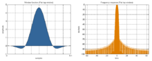
Hann window
 Hann window; B = 1.50Main article: Hann function
- Note that:
The ends of the cosine just touch zero, so the side-lobes roll off at about 18 dB per octave.[7]
The Hann and Hamming windows, both of which are in the family known as "raised cosine" or "generalized Hamming" windows, are respectively named after Julius von Hann and Richard Hamming. The term "Hanning window" is sometimes used to refer to the Hann window.
Hamming window
 Hamming window; B=1.37
The "raised cosine" with these particular coefficients was proposed by Richard W. Hamming. The window is optimized to minimize the maximum (nearest) side lobe, giving it a height of about one-fifth that of the Hann window, a raised cosine with simpler coefficients.[8][9]
- Note that:
Tukey window
 Tukey window, α=0.5; B=1.22
![w(n) = \left\{ \begin{matrix}
\frac{1}{2} \left[1+\cos \left(\pi \left( \frac{2 n}{\alpha (N-1)}-1 \right) \right) \right]
& \mbox{when}\, 0 \leqslant n \leqslant \frac{\alpha (N-1)}{2} \\ [0.5em]
1 & \mbox{when}\, \frac{\alpha (N-1)}{2}\leqslant n \leqslant (N-1) (1 - \frac{\alpha}{2}) \\ [0.5em]
\frac{1}{2} \left[1+\cos \left(\pi \left( \frac{2 n}{\alpha (N-1)}- \frac{2}{\alpha} + 1 \right) \right) \right]
& \mbox{when}\, (N-1) (1 - \frac{\alpha}{2}) \leqslant n \leqslant (N-1) \\
\end{matrix} \right.](c/c6c5993506eb86f322a7bf4b37743804.png)
The Tukey window,[10][11] also known as the tapered cosine window, can be regarded as a cosine lobe of width
 that is convolved with a rectangle window of width
  At α=0 it becomes rectangular, and at α=1 it becomes a Hann window.
Cosine window
 Cosine window; B=1.24
- also known as sine window
- cosine window describes the shape of
Lanczos window
 Sinc or Lanczos window; B=1.31
- used in Lanczos resampling
- for the Lanczos window, sinc(x) is defined as sin(πx)/(πx)
- also known as a sinc window, because:
-
 is the main lobe of a normalized sinc function
Triangular windows
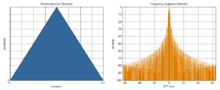 Bartlett window; B=1.33
Bartlett window with zero-valued end-points:
 Triangular window; B=1.33
With non-zero end-points:
Can be seen as the convolution of two half-sized rectangular windows, giving it a main lobe width of twice the width of a regular rectangular window. The nearest lobe is -26 dB down from the main lobe.[12]
Gaussian windows
 Gauss window, σ=0.4; B=1.45
The frequency response of a Gaussian is also a Gaussian (it is an eigenfunction of the Fourier Transform). Since the Gaussian function extends to infinity, it must either be truncated at the ends of the window, or itself windowed with another zero-ended window.[13]
Since the log of a Gaussian produces a parabola, this can be used for exact quadratic interpolation in frequency estimation.[14][15][16]
Bartlett–Hann window
 Bartlett-Hann window; B=1.46
Blackman windows
 Blackman window; α = 0.16; B=1.73
Blackman windows are defined as:[note 2]
By common convention, the unqualified term Blackman window refers to α=0.16.
Kaiser windows
 Kaiser window, α =2; B=1.5
 Kaiser window, α =3; B=1.8Main article: Kaiser window
A simple approximation of the DPSS window using Bessel functions, discovered by Jim Kaiser.[17][18]
where I0 is the zero-th order modified Bessel function of the first kind, and usually α = 3.
- Note that:
Low-resolution (high-dynamic-range) windows
Nuttall window, continuous first derivative
 Nuttall window, continuous first derivative; B=2.02
Blackman–Harris window
 Blackman–Harris window; B=2.01
A generalization of the Hamming family, produced by adding more shifted sinc functions, meant to minimize side-lobe levels[19][20]
Blackman–Nuttall window
 Blackman–Nuttall window; B=1.98
Flat top window
 Flat top window; B=3.77
Other windows
Bessel window
Dolph-Chebyshev window
Minimizes the Chebyshev norm of the side-lobes for a given main lobe width.[21]
Hann-Poisson window
A Hann window multiplied by a Poisson window, which has no side-lobes, in the sense that the frequency response drops off forever away from the main lobe. It can thus be used in hill climbing algorithms like Newton's method.[22]
Exponential or Poisson window
 Exponential window, τ=N/2, B=1.08
 Exponential window, τ=(N/2)/(60/8.69), B=3.46
The Poisson window, or more generically the exponential window increases exponentially towards the center of the window and decreases exponentially in the second half. Since the exponential function never reaches zero, the values of the window at its limits are non-zero (it can be seen as the multiplication of an exponential function by a rectangular window [23]). It is defined by
where τ is the time constant of the function. The exponential function decays as e = 2.71828 or approximately 8.69 dB per time constant.[24] This means that for a targetted decay of D dB over half of the window length, the time constant τ is given by
Rife-Vincent window
DPSS or Slepian window
The DPSS (digital prolate spheroidal sequence) or Slepian window is used to maximize the energy concentration in the main lobe.[25]
Comparison of windows
 Stopband attenuation of different windows
When selecting an appropriate window function for an application, this comparison graph may be useful. The graph shows only the main lobe of the window's frequency response in detail. Beyond that only the envelope of the sidelobes is shown to reduce clutter. The frequency axis has units of FFT "bins" when the window of length N is applied to data and a transform of length N is computed. For instance, the value at frequency ½ "bin" is the response that would be measured in bins k and k+1 to a sinusoidal signal at frequency k+½. It is relative to the maximum possible response, which occurs when the signal frequency is an integer number of bins. The value at frequency ½ is referred to as the maximum scalloping loss of the window, which is one metric used to compare windows. The rectangular window is noticeably worse than the others in terms of that metric.
Other metrics that can be seen are the width of the main lobe and the peak level of the sidelobes, which respectively determine the ability to resolve comparable strength signals and disparate strength signals. The rectangular window (for instance) is the best choice for the former and the worst choice for the latter. What cannot be seen from the graphs is that the rectangular window has the best noise bandwidth, and despite its 3 dB potential scalloping loss, it is the best choice for detecting a sinusoid at low signal-to-noise ratios.
Overlapping windows
When the length of a data set to be transformed is larger than necessary to provide the desired frequency resolution, a common practice is to subdivide it into smaller sets and window them individually. To mitigate the "loss" at the edges of the window, the individual sets may overlap in time. See Welch method of power spectral analysis and the Modified discrete cosine transform.
See also
- Multitaper
- Apodization
- Welch method
- Short-time Fourier transform
- Window design method
Notes
- ^ This produces an asymmetric form known as "DFT-even" or "periodic".
- ^ a b c d e f g h Windows of the form:
References
- ^ Eric W. Weisstein (2003). CRC Concise Encyclopedia of Mathematics. CRC Press. ISBN 1584883472. http://books.google.com/?id=aFDWuZZslUUC&pg=PA97&dq=apodization+function.
- ^ Carlo Cattani and Jeremiah Rushchitsky (2007). Wavelet and Wave Analysis As Applied to Materials With Micro Or Nanostructure. World Scientific. ISBN 9812707840. http://books.google.com/?id=JuJKu_0KDycC&pg=PA53&dq=define+%22window+function%22+nonzero+interval.
- ^ Curtis Roads (2002). Microsound. MIT Press. ISBN 0262182157.
- ^ Mastering Windows: Improving Reconstruction
- ^ https://ccrma.stanford.edu/~jos/sasp/Properties.html
- ^ https://ccrma.stanford.edu/~jos/sasp/Rectangular_window_properties.html
- ^ https://ccrma.stanford.edu/~jos/sasp/Hann_or_Hanning_or.html
- ^ Loren D. Enochson and Robert K. Otnes (1968). Programming and Analysis for Digital Time Series Data. U.S. Dept. of Defense, Shock and Vibration Info. Center. pp. 142. http://books.google.com/?id=duBQAAAAMAAJ&q=%22hamming+window%22+date:0-1970&dq=%22hamming+window%22+date:0-1970.
- ^ https://ccrma.stanford.edu/~jos/sasp/Hamming_Window.html
- ^ Tukey, J.W. (1967). "An introduction to the calculations of numerical spectrum analysis". Spectral Analysis of Time Series: 25–46
- ^ Harris, F.J. (1978). "On the use of windows for harmonic analysis with the discrete Fourier transform". Proceedings of the IEEE 66: 51–83. doi:10.1109/PROC.1978.10837.
- ^ https://ccrma.stanford.edu/~jos/sasp/Properties_I_I_I.html
- ^ https://ccrma.stanford.edu/~jos/sasp/Gaussian_Window_Transform.html
- ^ https://ccrma.stanford.edu/~jos/sasp/Matlab_Gaussian_Window.html
- ^ https://ccrma.stanford.edu/~jos/sasp/Quadratic_Interpolation_Spectral_Peaks.html
- ^ https://ccrma.stanford.edu/~jos/sasp/Gaussian_Window_Transform_I.html
- ^ https://ccrma.stanford.edu/~jos/sasp/Kaiser_Window.html
- ^ https://ccrma.stanford.edu/~jos/sasp/Kaiser_DPSS_Windows_Compared.html
- ^ https://ccrma.stanford.edu/~jos/sasp/Blackman_Harris_Window_Family.html
- ^ https://ccrma.stanford.edu/~jos/sasp/Three_Term_Blackman_Harris_Window.html
- ^ https://ccrma.stanford.edu/~jos/sasp/Dolph_Chebyshev_Window.html
- ^ https://ccrma.stanford.edu/~jos/sasp/Hann_Poisson_Window.html
- ^ Smith, Julius O. III (April 23), Spectral Audio Signal Processing, https://ccrma.stanford.edu/~jos/sasp/Poisson_Window.html, retrieved November 22 2011
- ^ Gade, Svend; Herlufsen, Henrik (1987). "Technical Review No 3-1987: Windows to FFT analysis (Part I)". Brüel & Kjær. http://www.bksv.com/doc/Bv0031.pdf. Retrieved November 22 2011.
- ^ https://ccrma.stanford.edu/~jos/sasp/Slepian_DPSS_Window.html
Other references
- Harris, Fredric j. (January 1978). "On the use of Windows for Harmonic Analysis with the Discrete Fourier Transform". Proceedings of the IEEE 66 (1): 51–83. doi:10.1109/PROC.1978.10837. http://web.mit.edu/xiphmont/Public/windows.pdf. Article on FFT windows which introduced many of the key metrics used to compare windows.
- Nuttall, Albert H. (February 1981). "Some Windows with Very Good Sidelobe Behavior". IEEE Transactions on Acoustics, Speech, and Signal Processing 29 (1): 84–91. doi:10.1109/TASSP.1981.1163506. Extends Harris' paper, covering all the window functions known at the time, along with key metric comparisons.
- Oppenheim, Alan V.; Schafer, Ronald W.; Buck, John A. (1999). Discrete-time signal processing. Upper Saddle River, N.J.: Prentice Hall. pp. 468–471. ISBN 0-13-754920-2.
- Bergen, S.W.A.; A. Antoniou (2004). "Design of Ultraspherical Window Functions with Prescribed Spectral Characteristics". EURASIP Journal on Applied Signal Processing 2004 (13): 2053–2065. doi:10.1155/S1110865704403114.
- Bergen, S.W.A.; A. Antoniou (2005). "Design of Nonrecursive Digital Filters Using the Ultraspherical Window Function". EURASIP Journal on Applied Signal Processing 2005 (12): 1910–1922. doi:10.1155/ASP.2005.1910.
- US patent 7065150, Park, Young-Seo, "System and method for generating a root raised cosine orthogonal frequency division multiplexing (RRC OFDM) modulation", published 2003, issued 2006
- LabView Help, Characteristics of Smoothing Filters, http://zone.ni.com/reference/en-XX/help/371361B-01/lvanlsconcepts/char_smoothing_windows/
- Evaluation of Various Window Function using Multi-Instrument, http://www.multi-instrument.com/doc/D1003/Evaluation_of_Various_Window_Functions_using_Multi-Instrument_D1003.pdf
Categories:- Statistical theory
- Data analysis
- Time series analysis
- Fourier analysis
- Signal processing
- Digital signal processing
- Types of functions


Wikimedia Foundation. 2010.