- Maximum a posteriori estimation
-
In Bayesian statistics, a maximum a posteriori probability (MAP) estimate is a mode of the posterior distribution. The MAP can be used to obtain a point estimate of an unobserved quantity on the basis of empirical data. It is closely related to Fisher's method of maximum likelihood (ML), but employs an augmented optimization objective which incorporates a prior distribution over the quantity one wants to estimate. MAP estimation can therefore be seen as a regularization of ML estimation.
Contents
Description
Assume that we want to estimate an unobserved population parameter θ on the basis of observations x. Let f be the sampling distribution of x, so that f(x | θ) is the probability of x when the underlying population parameter is θ. Then the function
is known as the likelihood function and the estimate
is the maximum likelihood estimate of θ.
Now assume that a prior distribution g over θ exists. This allows us to treat θ as a random variable as in Bayesian statistics. Then the posterior distribution of θ is as follows:
where g is density function of θ, Θ is the domain of g. This is a straightforward application of Bayes' theorem.
The method of maximum a posteriori estimation then estimates θ as the mode of the posterior distribution of this random variable:
The denominator of the posterior distribution (so-called partition function) does not depend on θ and therefore plays no role in the optimization. Observe that the MAP estimate of θ coincides with the ML estimate when the prior g is uniform (that is, a constant function). The MAP estimate is a limit of Bayes estimators under a sequence of 0-1 loss functions, but generally not a Bayes estimator per se, unless θ is discrete.[citation needed]
Computing
MAP estimates can be computed in several ways:
- Analytically, when the mode(s) of the posterior distribution can be given in closed form. This is the case when conjugate priors are used.
- Via numerical optimization such as the conjugate gradient method or Newton's method. This usually requires first or second derivatives, which have to be evaluated analytically or numerically.
- Via a modification of an expectation-maximization algorithm. This does not require derivatives of the posterior density.
- Via a Monte Carlo method using simulated annealing
Criticism
While MAP estimation is a limit of Bayes estimators (under the 0-1 loss function), it is not very representative of Bayesian methods in general. This is because MAP estimates are point estimates, whereas Bayesian methods are characterized by the use of distributions to summarize data and draw inferences: thus, Bayesian methods tend to report the posterior mean or median instead, together with credible intervals. This is both because these estimators are optimal under squared-error and linear-error loss respectively - which are more representative of typical loss functions - and because the posterior distribution may not have a simple analytic form: in this case, the distribution can be simulated using Markov chain Monte Carlo techniques, while optimization to find its mode(s) may be difficult or impossible.
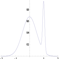 An example of a density of a bimodal distribution in which the highest mode is uncharacteristic of the majority of the distribution
In many types of models, such as mixture models, the posterior may be multi-modal. In such a case, the usual recommendation is that one should choose the highest mode: this is not always feasible (global optimization is a difficult problem), nor in some cases even possible (such as when identifiability issues arise). Furthermore, the highest mode may be uncharacteristic of the majority of the posterior.
Finally, unlike ML estimators, the MAP estimate is not invariant under reparameterization. Switching from one parameterization to another involves introducing a Jacobian that impacts on the location of the maximum.[citation needed]
As an example of the difference between Bayes estimators mentioned above (mean and median estimators) and using an MAP estimate, consider the case where there is a need to classify inputs x as either positive or negative (for example, loans as risky or safe). Suppose there are just three possible hypotheses about the correct method of classification h1, h2 and h3 with posteriors 0.4, 0.3 and 0.3 respectively. Suppose given a new instance, x, h1 classifies it as positive, whereas the other two classify it as negative. Using the MAP estimate for the correct classifier h1, x is classified as positive, whereas the Bayes estimators would average over all hypotheses and classify x as negative.
Example
Suppose that we are given a sequence
 of IID
  random variables and an a priori distribution of μ is given by
  . We wish to find the MAP estimate of μ.
The function to be maximized is then given by
which is equivalent to minimizing the following function of μ:
Thus, we see that the MAP estimator for μ is given by
which turns out to be a linear interpolation between the prior mean and the sample mean weighted by their respective covariances.
The case of
 is called a non-informative prior and leads to an ill-defined a priori probability distribution; in this case
References
- M. DeGroot, Optimal Statistical Decisions, McGraw-Hill, (1970).
- Harold W. Sorenson, (1980) "Parameter Estimation: Principles and Problems", Marcel Dekker.
Categories:- Estimation theory
- Bayesian inference
- Statistical theory
- Logic and statistics


Wikimedia Foundation. 2010.